To demonstrate the regression metrics, a simple linear regression model will be trained. Importing the libraries:

In [2]:

import numpy as np
import matplotlib.pyplot as plt
from sklearn.datasets import make_regression
from sklearn.model_selection import train_test_split
from sklearn.linear_model import LinearRegression
from sklearn.metrics import mean_absolute_error, mean_squared_error

Making a simple regression dataset.

In [4]:

X, y = make_regression(n_samples=200, n_features=1, noise=15, random_state=42)
X_train, X_test, y_train, y_test = train_test_split(X, y, test_size=0.3, random_state=42)

Fitting the model.

In [6]:

model = LinearRegression()
model.fit(X_train, y_train)

y_pred = model.predict(X_test)

Calculating and printing the metrics.

In [8]:

mae = mean_absolute_error(y_test, y_pred)
mse = mean_squared_error(y_test, y_pred)
rmse = np.sqrt(mse)

print("--- Regression Metrics ---")
print(f"MAE:  {mae:.4f}")
print(f"MSE:  {mse:.4f}")
print(f"RMSE: {rmse:.4f}")

--- Regression Metrics ---
MAE:  12.6289
MSE:  261.5702
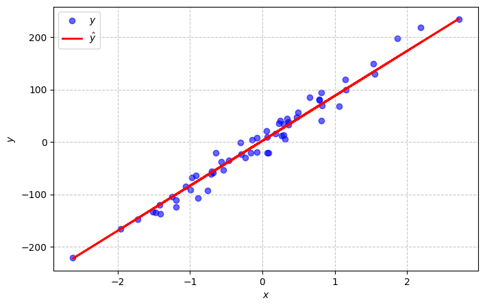
RMSE: 16.1731

Visualizing the predictions.

In [10]:

plt.figure(figsize=(8, 5))
plt.scatter(X_test, y_test, color='blue', alpha=0.6, label=r'$y$')
plt.plot(X_test, y_pred, color='red', linewidth=2, label=r'$\hat{y}$')
plt.xlabel("$x$")
plt.ylabel("$y$")
plt.legend()
plt.grid(True, linestyle='--', alpha=0.7)
plt.show()