In [1]:

---
execute:
  eval: false
  echo: true
  warning: false
format:
  html:
    code-fold: false
---

Importing the libraries for a logistic regression.

In [6]:

import numpy as np
import matplotlib.pyplot as plt
from sklearn.linear_model import LogisticRegression

Generating the data.

In [7]:

np.random.seed(42)
X = np.random.normal(0, 2, 100).reshape(-1, 1)
y = (X[:, 0] > 0).astype(int)
flip_idx = np.random.choice(100, size=10, replace=False)
y[flip_idx] = 1 - y[flip_idx]

Creating and fitting the model.

In [8]:

model = LogisticRegression()
model.fit(X, y)

LogisticRegression()

In a Jupyter environment, please rerun this cell to show the HTML representation or trust the notebook.
On GitHub, the HTML representation is unable to render, please try loading this page with nbviewer.org.

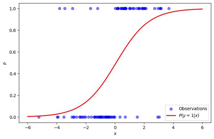
Plotting the final result.

In [12]:

X_test = np.linspace(-6, 6, 300).reshape(-1, 1)
probabilities = model.predict_proba(X_test)[:, 1]

plt.figure(figsize=(8, 5))
plt.scatter(X, y, color='blue', alpha=0.5, label='Observations')
plt.plot(X_test, probabilities, color='red', linewidth=2, label=r'$P(y=1 | x)$')

plt.xlabel("x")
plt.ylabel("P")
plt.legend()
plt.show()