---
execute:
  eval: false
  echo: true
  warning: false
format:
  html:
    code-fold: false
---In [1]:
Importing libraries for the SR.
In [1]:
import numpy as np
import matplotlib.pyplot as plt
from gplearn.genetic import SymbolicRegressor
import graphviz
Creating a function and drawing noisy observations from it.
In [2]:
def true_law(X):
    return X[:, 0]**2 - 0.5 * np.cos(X[:, 1])

rng = np.random.RandomState(42)
X_train = rng.uniform(-2, 2, size=(200, 2))
y_train = true_law(X_train) + rng.normal(0, 0.05, size=200)

X_test = rng.uniform(-2, 2, size=(100, 2))
y_test = true_law(X_test)
Training the model.
In [3]:
est_gp = SymbolicRegressor(population_size=2000,
                           generations=20, stopping_criteria=0.01,
                           p_crossover=0.7, p_subtree_mutation=0.1,
                           p_hoist_mutation=0.05, p_point_mutation=0.1,
                           max_samples=0.9, verbose=1,
                           parsimony_coefficient=0.01, random_state=42,
                           function_set=('add', 'sub', 'mul', 'div', 'cos', 'sin'))

est_gp.fit(X_train, y_train)
| Population Average | Best Individual |
---- ------------------------- ------------------------------------------ ----------
Gen Length Fitness Length Fitness OOB Fitness Time Left
0 19.73 8.28841 7 0.272313 0.24835 40.18s
1 6.58 1.34506 3 0.263839 0.324619 28.90s
2 7.22 1.34527 7 0.218505 0.243268 29.24s
3 5.76 1.62976 7 0.195336 0.17832 25.15s
4 3.74 0.880664 7 0.187003 0.253322 22.72s
5 4.97 0.908279 8 0.182972 0.204203 25.31s
6 6.25 1.08844 10 0.0501441 0.0485609 52.23s
7 7.09 1.05202 10 0.0491968 0.0570867 28.55s
8 7.43 1.01999 10 0.0484214 0.0640652 19.02s
9 8.15 0.893839 11 0.0474426 0.0550371 16.43s
10 9.34 0.747861 11 0.0459216 0.0687259 24.57s
11 9.98 0.739079 11 0.0451721 0.0754717 47.72s
12 10.01 0.859513 11 0.0463533 0.064841 11.92s
13 10.05 0.627553 11 0.0454762 0.0727347 9.92s
14 10.08 0.73443 13 0.0447408 0.0338422 8.99s
15 9.97 0.746023 11 0.0466114 0.0625181 6.54s
16 9.82 0.679483 11 0.0458664 0.0692227 4.97s
17 10.24 0.935914 9 0.0426343 0.03541 5.55s
18 9.95 0.65024 9 0.04105 0.0496688 1.74s
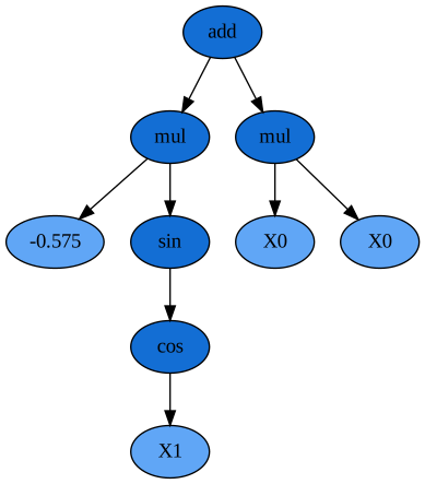
19 9.94 3.09489 9 0.0402459 0.0569062 0.00sadd(mul(-0.575, sin(cos(X1))), mul(X0, X0))In a Jupyter environment, please rerun this cell to show the HTML representation or trust the notebook.
On GitHub, the HTML representation is unable to render, please try loading this page with nbviewer.org.
Parameters
| population_size | 2000 | |
| generations | 20 | |
| tournament_size | 20 | |
| stopping_criteria | 0.01 | |
| const_range | (-1.0, ...) | |
| init_depth | (2, ...) | |
| init_method | 'half and half' | |
| function_set | ('add', ...) | |
| metric | 'mean absolute error' | |
| parsimony_coefficient | 0.01 | |
| p_crossover | 0.7 | |
| p_subtree_mutation | 0.1 | |
| p_hoist_mutation | 0.05 | |
| p_point_mutation | 0.1 | |
| p_point_replace | 0.05 | |
| max_samples | 0.9 | |
| feature_names | None | |
| warm_start | False | |
| low_memory | False | |
| n_jobs | 1 | |
| verbose | 1 | |
| random_state | 42 |
Plotting the prediction against the true values, and printing the best equation found.
In [7]:
print("y = X0^2 - 0.5*cos(X1)")
print("y_hat = ", est_gp._program)
print()

y_gp = est_gp.predict(X_test)

plt.figure(figsize=(8, 6))
plt.scatter(y_test, y_gp, alpha=0.6, color='blue', edgecolor='k')
plt.plot([y_test.min(), y_test.max()], [y_test.min(), y_test.max()], 'r--', lw=2, label=r"$\hat y = y$")
plt.xlabel(r"$y$")
plt.ylabel(r"$\hat y$")
plt.legend()
plt.show()
y = X0^2 - 0.5*cos(X1)
y_hat = add(mul(-0.575, sin(cos(X1))), mul(X0, X0))
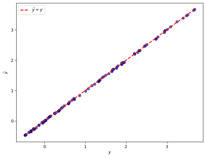
Showing the tree structure.
In [9]:
dot_data = est_gp._program.export_graphviz()
graph = graphviz.Source(dot_data)
graph