svm

In [1]:

---
execute:
  eval: false
  echo: true
  warning: false
format:
  html:
    code-fold: false
---

Importing packages for the SVM.

In [40]:

import numpy as np
import matplotlib.pyplot as plt
from sklearn.datasets import make_circles
from sklearn.svm import SVC
from sklearn.model_selection import train_test_split
from sklearn.preprocessing import StandardScaler
from sklearn.metrics import classification_report

Creating a synthetic classification dataset which is not linearly separable and normalizing the features.

In [42]:

X, y = make_circles(n_samples=150, factor=0.5, noise=0.1, random_state=42)
X_train, X_test, y_train, y_test = train_test_split(X, y, test_size=0.3, random_state=42)

scaler = StandardScaler()
X_train_scaled = scaler.fit_transform(X_train)
X_test_scaled = scaler.transform(X_test)

Creating one linear model and one model with RBF.

In [44]:

svm_linear = SVC(kernel='linear', C=1.0).fit(X_train_scaled, y_train)
svm_rbf = SVC(kernel='rbf', C=1.0, gamma='auto').fit(X_train_scaled, y_train)

Plotting the decision boundaries of each model.

In [47]:

def plot_svm_boundary(model, X, y, ax, title):
    ax.scatter(X[:, 0], X[:, 1], c=y, cmap='bwr', s=30, zorder=3)

    xlim = ax.get_xlim()
    ylim = ax.get_ylim()
    xx = np.linspace(xlim[0], xlim[1], 100)
    yy = np.linspace(ylim[0], ylim[1], 100)
    YY, XX = np.meshgrid(yy, xx)
    xy = np.vstack([XX.ravel(), YY.ravel()]).T

    Z = model.decision_function(xy).reshape(XX.shape)

    ax.contour(XX, YY, Z, colors='k', levels=[-1, 0, 1], alpha=0.5,
               linestyles=['--', '-', '--'])

    ax.scatter(model.support_vectors_[:, 0], model.support_vectors_[:, 1], s=100,
               linewidth=1, facecolors='none', edgecolors='k', label='Support Vectors')

    ax.set_title(title)
    ax.legend(loc='upper right')
    ax.set_xlabel(r"$x_1$")
    ax.set_ylabel(r"$x_2$")

fig, axes = plt.subplots(1, 2, figsize=(14, 6))

plot_svm_boundary(svm_linear, X_train_scaled, y_train, axes[0], "Linear SVM")
plot_svm_boundary(svm_rbf, X_train_scaled, y_train, axes[1], "RBF SVM")

plt.tight_layout()
plt.show()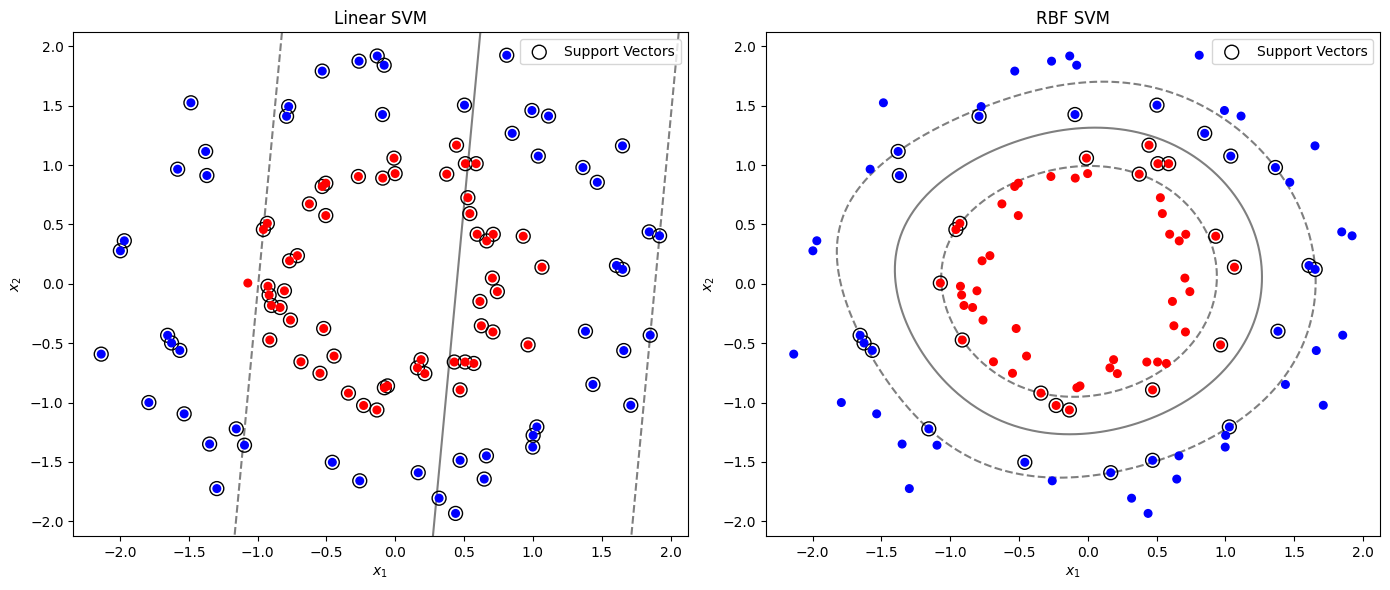

Printing the classifications reports of each model.

In [48]:

y_pred_linear = svm_linear.predict(X_test_scaled)
y_pred_rbf = svm_rbf.predict(X_test_scaled)

rep_linear = classification_report(y_test, y_pred_linear)
rep_rbf = classification_report(y_test, y_pred_rbf)

print("Linear")
print(rep_linear)
print(60*"=")
print("RBF")
print(rep_rbf)
print(60*"=")

Linear
              precision    recall  f1-score   support

           0       0.50      0.35      0.41        23
           1       0.48      0.64      0.55        22

    accuracy                           0.49        45
   macro avg       0.49      0.49      0.48        45
weighted avg       0.49      0.49      0.48        45

============================================================
RBF
              precision    recall  f1-score   support

           0       1.00      1.00      1.00        23
           1       1.00      1.00      1.00        22

    accuracy                           1.00        45
   macro avg       1.00      1.00      1.00        45
weighted avg       1.00      1.00      1.00        45

============================================================

As it was shown in the plot, the linear SVM was not able to separate the classes, while the RBF SVM was able to separate the observations.

svm.ipynb