import torch
import torch.nn as nn
import torch.optim as optim
from torchvision import datasets, transforms
from torch.utils.data import DataLoader

from sklearn.metrics import classification_report, confusion_matrix
import seaborn as sns
import numpy as np

import matplotlib.pyplot as plt1.1 Neural Networks (NNs)
Deep Learning (DL) is a subarea of Machine Learning (ML) based on models composed of artificial Neural Networks (NNs) (LeCun, Bengio, and Hinton 2015). These architectures are general function approximators inspired by biological neural processing (Prince 2023). The foundation of NNs began with the mathematical model of the biological neuron (McCulloch and Pitts 1943). This later inspired the Perceptron (Rosenblatt 1958), depicted in Figure 1. The Perceptron introduced learnable parameters composed of weights \(\boldsymbol{w}\in\mathbb R^n\) and a bias \(b\in \mathbb R\). Given an input \(\boldsymbol{x} \in \mathbb R^n\), the output \(\hat{y} \in \mathbb R\) of the Perceptron was defined as: \[ \hat{y} = f\left(b + \sum_{i=1}^n w_i x_i\right) = f\left(\boldsymbol{w}^T \boldsymbol{x} + b\right), \tag{1}\] where \(f(z) = \text{sgn}(z)\) was a step function.
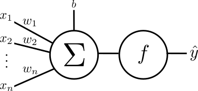
Following the Perceptron, the Adaptive Linear Element (Adaline) (Widrow and Hoff 1960) introduced a way to update weights using continuous activations during training. This model defined a loss function: \[ \mathcal L(\boldsymbol{w}, b) = \frac{1}{2} \left[y - (\boldsymbol{w}^T \boldsymbol{x} + b)\right]^2, \tag{2}\] allowing weights to be updated via the Delta Rule: \[ \boldsymbol{w}^{(k+1)} = \boldsymbol{w}^{(k)} + \eta \left[y_i - (\boldsymbol{w}^T \boldsymbol{x} + b)\right] \boldsymbol{x}. \tag{3}\]
Despite early successes, single-layer models were limited because they could only solve linearly separable problems (Minsky and Papert 2017). To overcome this limitation, step functions were replaced with differentiable non-linear functions, enabling the development of the backpropagation algorithm (Rumelhart, Hinton, and Williams 1986). Backpropagation employed chain rule to update parameters across stacked hidden layers, giving rise to the Multilayer Perceptron (MLP). Shortly after, the Universal Approximation Theorem (Cybenko 1989; Hornik 1991) established that a feedforward network with a single hidden layer containing a finite number of neurons could approximate any continuous function on compact subsets of \(\mathbb{R}^n\) under some assumptions.
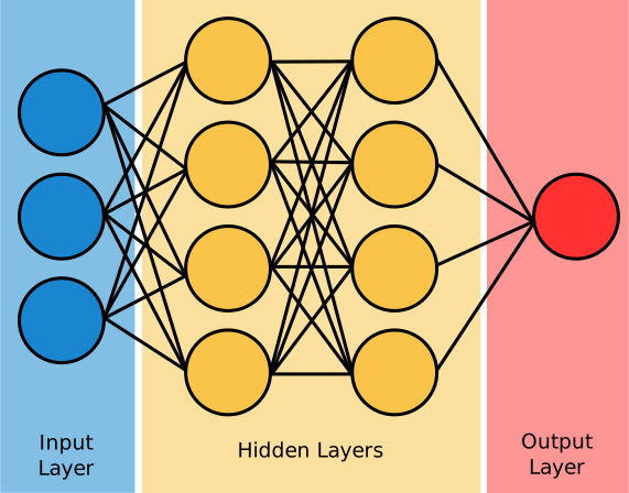
The foundational building block of modern deep architectures remains the artificial neuron. A single neuron receives an input vector \(\boldsymbol{x} \in \mathbb{R}^n\), computes an affine combination, and applies a non-linear activation function \(\sigma : \mathbb{R} \to \mathbb{R}\): \[ \hat{y} = \sigma\left(b + \sum_{i=1}^n w_i x_i\right) = \sigma\left(\boldsymbol{w}^T \boldsymbol{x} + b\right), \tag{4}\] where \(\boldsymbol{w} \in \mathbb{R}^n\) represents the weight vector and \(b \in \mathbb{R}\) denotes the scalar bias. The parameters \(\boldsymbol{\Theta} = \{\boldsymbol{w}, b\}\) constitute the learnable components of the unit. To approximate more complex function, neurons are organized in parallel to form a layer. A single layer mapping an input vector \(\boldsymbol{x} \in \mathbb{R}^n\) to an \(m\)-dimensional representation is defined as: \[ \boldsymbol{\hat{y}} = \sigma\left(\boldsymbol{W}\boldsymbol{x} + \boldsymbol{b}\right), \tag{5}\] where \(\boldsymbol{W} \in \mathbb{R}^{m \times n}\) is the linear coefficient matrix, \(\boldsymbol{b} \in \mathbb{R}^m\) is the bias vector and \(\boldsymbol{\hat{y}} \in \mathbb{R}^m\) is the output vector. Expanding this operation into matrix notation yields: \[ \begin{bmatrix} \hat{y}_1 \\ \hat{y}_2 \\ \vdots \\ \hat{y}_m \end{bmatrix} = \sigma \left( \begin{bmatrix} w_{11} & w_{12} & \cdots & w_{1n} \\ w_{21} & w_{22} & \cdots & w_{2n} \\ \vdots & \vdots & \ddots & \vdots \\ w_{m1} & w_{m2} & \cdots & w_{mn} \end{bmatrix} \begin{bmatrix} x_1 \\ x_2 \\ \vdots \\ x_n \end{bmatrix} + \begin{bmatrix} b_1 \\ b_2 \\ \vdots \\ b_m \end{bmatrix} \right). \tag{6}\] The activation function \(\sigma(\cdot)\) is applied element-wise. In an MLP, multiple layers are composed sequentially to parameterize a function \(f_{\boldsymbol{\Theta}}: \mathcal{X} \to \mathcal{Y}\) that maps the input space \(\mathcal{X}\) to the target space \(\mathcal{Y}\). Intermediate layers between input and output are called hidden layers. Figure 2 depicts a diagram of the MLP architecture.
The learnable parameters are optimized in a Supervised Learning framework using a labeled dataset \(\mathcal{D} = \{(\boldsymbol{x}_i, \boldsymbol{y}_i)\}_{i=1}^N\). Given a loss function \(\mathcal{L} : \mathcal Y \times \mathcal Y \to \mathbb R\), the learnable parameter set \(\boldsymbol{\Theta} = \{\boldsymbol{W}^{(l)}, \boldsymbol{b}^{(l)}\}_{l=1}^L\) is updated iteratively via backpropagation: \[ \boldsymbol{\Theta}^{(k+1)} = \boldsymbol{\Theta}^{(k)} - \eta \nabla_{\boldsymbol{\Theta}^{(k)}} \mathcal{L}\left(\boldsymbol{y}_i, f_{\boldsymbol{\Theta}^{(k)}}(\boldsymbol{x}_i)\right), \tag{7}\] where \(k\) denotes the optimization step index and \(\eta \in \mathbb{R}^+\) represents the learning rate. Finally, the MLP has some important hyperparameters that need to be tuned: number of hidden layers \(L\), number of neurons in each hidden layer \(m^{(l)}\) for \(l \in \{1, \dots, L\}\), activation functions for each hidden layer \(\sigma^{(l)}\) for \(l \in \{1, \dots, L\}\).
Code
Here, a simple MLP will be trained in a classification task using the MNIST dataset – which contains images of hand-written digits. Importing the libraries.
Setting the device.
device = torch.device("cuda" if torch.cuda.is_available() else "cpu")
print(f"Using device: {device}")
Using device: cudaNormalizing and creating the dataloaders.
transform = transforms.Compose([
    transforms.ToTensor(),
    transforms.Normalize((0.1307,), (0.3081,)),
    transforms.Lambda(lambda x: torch.flatten(x))
])

train_dataset = datasets.MNIST('./data', train=True, download=True, transform=transform)
test_dataset = datasets.MNIST('./data', train=False, transform=transform)

train_loader = DataLoader(train_dataset, batch_size=64, shuffle=True)
test_loader = DataLoader(test_dataset, batch_size=1000, shuffle=False)
Creating and instantiating the MLP. A model with one hidden layer containing 128 neurons and ReLU activations will be used.
class MLP(nn.Module):
    def __init__(
            self,
            input_size=784,
            hidden_size=128,
            output_size=10
        ):
        super(MLP, self).__init__()

        self.classifier = nn.Sequential(
            nn.Linear(input_size, hidden_size),
            nn.ReLU(),
            nn.Linear(hidden_size, hidden_size),
            nn.ReLU(),
            nn.Linear(hidden_size, output_size)
        )

    def forward(self, x):
        return self.classifier(x)

    def fit(
            self,
            device,
            train_loader,
            optimizer,
            criterion,
            epochs
        ):
        self.train()
        self.train_loss = []

        for epoch in range(1, epochs + 1):
            epoch_loss = 0.0

            for data, target in train_loader:
                data, target = data.to(device), target.to(device)

                optimizer.zero_grad()
                output = self(data)
                loss = criterion(output, target)
                loss.backward()
                optimizer.step()

                epoch_loss += loss.item()

            avg_loss = epoch_loss / len(train_loader)
            self.train_loss.append(avg_loss)
            print(f"Epoch [{epoch}/{epochs}] | Average Loss: {avg_loss:.6f}")

model = MLP().to(device)

params = sum(p.numel() for p in model.parameters() if p.requires_grad)
print(f"Number of params: {params}")
Number of params: 118282Making the training loop.
criterion = nn.CrossEntropyLoss()
optimizer = optim.SGD(model.parameters(), lr=0.01)

model.fit(device, train_loader, optimizer, criterion, epochs=10)
Epoch [1/10] | Average Loss: 0.825505
Epoch [2/10] | Average Loss: 0.316130
Epoch [3/10] | Average Loss: 0.261313
Epoch [4/10] | Average Loss: 0.223332
Epoch [5/10] | Average Loss: 0.193474
Epoch [6/10] | Average Loss: 0.170477
Epoch [7/10] | Average Loss: 0.152012
Epoch [8/10] | Average Loss: 0.136417
Epoch [9/10] | Average Loss: 0.123799
Epoch [10/10] | Average Loss: 0.112818Plotting the training curve.
plt.plot(model.train_loss)
plt.xlabel("Epoch")
plt.ylabel("Cross-Entropy Loss")
plt.show()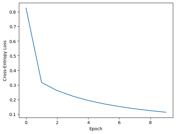
Calculating the metrics.
model.eval()
all_preds = []
all_targets = []

with torch.no_grad():
    for data, target in test_loader:
        data, target = data.to(device), target.to(device)
        output = model(data)
        preds = output.argmax(dim=1)

        all_preds.extend(preds.cpu().numpy())
        all_targets.extend(target.cpu().numpy())

print(classification_report(all_targets, all_preds, digits=4))
precision recall f1-score support
0 0.9660 0.9867 0.9763 980
1 0.9756 0.9850 0.9803 1135
2 0.9691 0.9738 0.9715 1032
3 0.9542 0.9703 0.9622 1010
4 0.9595 0.9654 0.9624 982
5 0.9638 0.9552 0.9595 892
6 0.9629 0.9749 0.9689 958
7 0.9666 0.9582 0.9624 1028
8 0.9755 0.9384 0.9566 974
9 0.9617 0.9445 0.9530 1009
accuracy 0.9656 10000
macro avg 0.9655 0.9652 0.9653 10000
weighted avg 0.9656 0.9656 0.9655 10000
Plotting the confusion matrix.
cm = confusion_matrix(all_targets, all_preds)

plt.figure(figsize=(7, 7))
sns.heatmap(
    cm,
    annot=True,
    fmt='d',
    cmap='Blues',
    cbar=False,
    xticklabels=range(10),
    yticklabels=range(10)
)
plt.xlabel("Predicted Label")
plt.ylabel("True Label")
plt.show()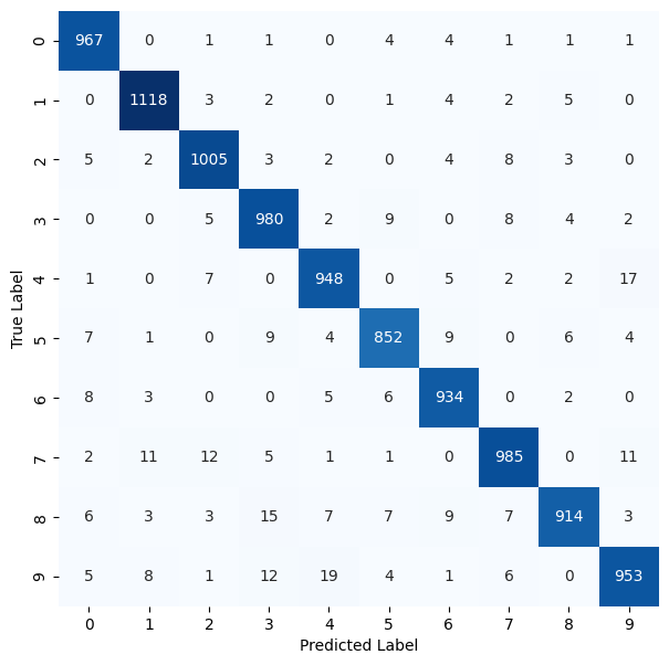
References
Cybenko, George. 1989. “Approximation by Superpositions of a Sigmoidal Function.” Mathematics of Control, Signals and Systems 2 (4): 303–14.
Hornik, Kurt. 1991. “Approximation Capabilities of Multilayer Feedforward Networks.” Neural Networks 4 (2): 251–57.
LeCun, Yann, Yoshua Bengio, and Geoffrey Hinton. 2015. Deep Learning. Nature. Vol. 521. 7553. Nature Publishing Group UK London.
McCulloch, Warren S, and Walter Pitts. 1943. “A Logical Calculus of the Ideas Immanent in Nervous Activity.” The Bulletin of Mathematical Biophysics 5 (4): 115–33.
Minsky, Marvin, and Seymour A Papert. 2017. Perceptrons: An Introduction to Computational Geometry. MIT Press.
Prince, Simon JD. 2023. Understanding Deep Learning. MIT press.
Rosenblatt, Frank. 1958. “The Perceptron: A Probabilistic Model for Information Storage and Organization in the Brain.” Psychological Review 65 (6): 386.
Rumelhart, David E, Geoffrey E Hinton, and Ronald J Williams. 1986. “Learning Representations by Back-Propagating Errors.” Nature 323 (6088): 533–36.
Widrow, Bernard, and Marcian E Hoff. 1960. “Adaptive Switching Circuits.” In IRE WESCON Convention Record.