import numpy as np
import matplotlib.pyplot as plt
from diffusers import DDPMScheduler, EulerDiscreteScheduler, ScoreSdeVeScheduler1.1.5. Elucidated Diffusion Models (EDMs)
After the Stochastic Differential Equations (SDEs) general framework for Diffusion Models (DMs), Elucidated Diffusion Models (EDMs) (Karras et al. 2022) focused on simplifying the diffusion framework, decoupling the choices of parametrization such as noise schedules and other important hyperparameters that were jointly defined in previous approaches.
Given the data distribution \(p_0(\boldsymbol x)\), with \(\boldsymbol x \in \mathbb R\), and its standard deviation \(\sigma_0 \in \mathbb R\), let \(p(\boldsymbol x, \sigma)\) denote a modified data distribution with noise scale \(\sigma \in \mathbb R\). Using the general Probability Flow ODE equation, EDM formulates diffusion with \(\boldsymbol{f}(\boldsymbol x, t) = \boldsymbol 0\) and \(g(t)^2 = 2 \frac{d\sigma(t)}{dt} \sigma(t)\), that is: \[ d\boldsymbol{x} = - \frac{d\sigma(t)}{dt} \sigma(t) \nabla_{\boldsymbol x} \log p(\boldsymbol x, \sigma(t)) dt, \tag{1}\] where \(\sigma(t) : \mathbb R \to \mathbb R\) is a noise scale. Running forward in time goes away from the data, while the opposite goes towards the data distribution. These choices imply that the diffusion process has no drift coefficient, therefore, the Markov chain only adds noise throughout the iterations.
Given a trained denoiser \(\boldsymbol{D}_{\boldsymbol{\theta}}(\boldsymbol{x}, \sigma(t)) : \mathbb R^{n \times 1} \to \mathbb R^n\), parametrized by \(\boldsymbol{\theta}\), that minimizes the expected \(\ell_2\) error to the clean data, the score function can be expressed in terms of the optimal denoiser \(\boldsymbol{D} : \mathbb R^{n \times 1} \to \mathbb R^n\): \[ \nabla_{\boldsymbol x} \log p(\boldsymbol x, \sigma(t)) = \frac{\boldsymbol{D}(\boldsymbol{x}, \sigma(t)) - \boldsymbol{x}}{\sigma(t)^2}. \tag{2}\] Substituting the denoiser into the Probability Flow ODE yields: \[ d\boldsymbol{x} = -\frac{d\sigma(t)}{dt} \frac{\boldsymbol{D}_{\boldsymbol{\theta}}(\boldsymbol{x}, \sigma(t)) - \boldsymbol{x}}{\sigma(t)} dt. \tag{3}\] In particular, EDM employed \(\sigma(t) = t\), simplifying the ODE to: \[ d\boldsymbol{x} = \frac{\boldsymbol{x} - \boldsymbol{D}_{\boldsymbol{\theta}}(\boldsymbol{x}, t)}{t} dt. \tag{4}\] This simplified the concept of time and noise, as both of these quantities represented the severity of data corruption.
To ensure training stability, EDM introduces a pre-conditioning framework that makes the neural network inputs scaled dynamically based on \(\sigma\) to maintain a zero mean and unit variance. This ensures the neural network architecture does not need to be adapted to a specific noise schedule. Finally, the model is trained by minimizing: \[ \mathcal{L}(\boldsymbol{\theta}) = \mathbb{E}_{\boldsymbol{x}, \boldsymbol{\epsilon}, \sigma} \left[ \lambda(\sigma) \left\| \boldsymbol{D}_{\boldsymbol{\theta}} (\boldsymbol{x} + \boldsymbol{\epsilon}, \sigma) - \boldsymbol{x} \right\|_2^2 \right], \tag{5}\] where the noise \(\boldsymbol{\epsilon} \in \mathbb R^n\) is sampled from \(\boldsymbol{\epsilon} \sim \mathcal{N}(\boldsymbol{0}, \sigma^2 \boldsymbol{I})\). The weighting function \(\lambda(\sigma) : \mathbb R \to \mathbb R\) is defined as: \[ \lambda(\sigma) = \frac{\sigma^2 + \sigma_0^2}{\sigma^2\cdot \sigma_0^2}. \tag{6}\] Overall, EDM simplified the design choices of implementing DMs, including the noise schedules, network pre-conditioning, among other practical aspects.
For sampling, EDM proposed a Stochastic Churn Sampler by using the Probability Flow ODE.
Code
Importing the packages.
Instantiating the schedulers.
num_steps = 100
normalized_time = np.linspace(0, 1, num_steps)

ddpm = DDPMScheduler(num_train_timesteps=1000, beta_schedule="linear")
ddpm.set_timesteps(num_steps)

edm = EulerDiscreteScheduler(num_train_timesteps=1000, use_karras_sigmas=True)
edm.set_timesteps(num_steps)

smld = ScoreSdeVeScheduler(num_train_timesteps=1000)
smld.set_timesteps(num_steps)
Extracting the noise schedules from each method.
alpha_bar = ddpm.alphas_cumprod.numpy()[ddpm.timesteps.numpy()][::-1]
alpha_ddpm = np.sqrt(alpha_bar)
sigma_ddpm = np.sqrt(1 - alpha_bar)

sigma_edm = edm.sigmas.numpy()[::-1][1:]
alpha_edm = np.ones_like(sigma_edm)

sigma_min = smld.config.sigma_min
sigma_max = smld.config.sigma_max
sigma_smld = sigma_min * (sigma_max / sigma_min) ** normalized_time
alpha_smld = np.ones_like(sigma_smld)

t_subvp = np.linspace(0.001, 0.999, num_steps)
alpha_subvp = 1 - t_subvp
sigma_subvp = t_subvp
Plotting the schedules.
def log_snr(alpha, sigma):
    return 2 * np.log(alpha / sigma)

plt.figure(figsize=(10, 6))

plt.plot(normalized_time, log_snr(alpha_ddpm, sigma_ddpm), label="VP SDE", linewidth=2, c="blue")
plt.plot(normalized_time, log_snr(alpha_edm, sigma_edm), label="EDM VE SDE", linewidth=2, c="orange")
plt.plot(normalized_time, log_snr(alpha_smld, sigma_smld), label="VE SDE", linewidth=2, linestyle='--', c="crimson")
plt.plot(normalized_time, log_snr(alpha_subvp, sigma_subvp), label="Sub-VP SDE", linewidth=2, c="purple")

plt.xlabel(r"$t$", fontsize=12)
plt.ylabel(r"$\log(\text{SNR})$", fontsize=12)
plt.grid(True, alpha=0.3)
plt.legend(fontsize=11)
plt.tight_layout()
plt.show()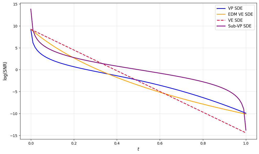
References
Karras, Tero, Miika Aittala, Timo Aila, and Samuli Laine. 2022. “Elucidating the Design Space of Diffusion-Based Generative Models.” Advances in Neural Information Processing Systems 35: 26565–77.