import numpy as np
import matplotlib.pyplot as plt
import seaborn as sns
from sklearn.datasets import load_digits
from sklearn.decomposition import PCA
from sklearn.manifold import TSNE
import umap3.1. Dimensionality Reduction
When analyzing high-dimensional data, it is not possible to visualize the data in order to observe its behavior. For that, some methods seek to reduce the dimensionality of the inputs to a lower-dimensional representation, keeping some aspects of the original data. Though used for visualization, these methods can also be helpful for reducing the number of input features to a supervised model.
Principal Component Analysis (PCA)
Principal Component Analysis (PCA) is a linear dimensionality reduction technique. It seeks to project the data onto a lower-dimensional subspace such that the variance of the projected data is maximized. Geometrically, this is equivalent to finding the orthogonal axes along which the data varies the most.
Let the dataset \(\mathcal{D} = \{\boldsymbol x_i\}_{i=1}^N\), where \(\boldsymbol x_i \in \mathbb R^n\), be centered, such that the mean of each feature is zero. The empirical covariance matrix \(\boldsymbol{\Sigma} \in \mathbb{R}^{n \times n}\) is given by: \[ \boldsymbol{\Sigma} = \frac{1}{N-1} \boldsymbol{X}^T \boldsymbol{X}. \tag{1}\] To find the first principal component \(\boldsymbol{w}_1 \in \mathbb{R}^n\), one looks to maximize the variance of the projection \(\boldsymbol{X}\boldsymbol{w}_1\), which is framed as a constrained optimization problem: \[ \max_{\boldsymbol{w}_1} \boldsymbol{w}_1^T \boldsymbol{\Sigma} \boldsymbol{w}_1 \quad \text{subject to} \quad \|\boldsymbol{w}_1\|_2 = 1. \tag{2}\] Using Lagrange multipliers, the optimization simplifies to an eigenvalue problem: \[ \boldsymbol{\Sigma} \boldsymbol{w}_1 = \lambda_1 \boldsymbol{w}_1. \tag{3}\] The optimal weight vector \(\boldsymbol{w}_1\) is the eigenvector corresponding to the largest eigenvalue \(\lambda_1\) of the covariance matrix. Subsequent principal components are found by calculating the remaining eigenvectors, ordered by the magnitude of their respective eigenvalues in descending order. The final low-dimensional representation is obtained by projecting \(\boldsymbol{X}\) onto the matrix containing the first \(k\) eigenvectors.
\(t\)-Distributed Stochastic Neighborhood Embedding (\(t\)-SNE)
\(t\)-Distributed Stochastic Neighborhood Embedding (\(t\)-SNE) (Van der Maaten and Hinton 2008) is a non-linear dimensionality reduction technique. First, it converts high-dimensional Euclidean distances between data points into conditional probabilities that represent similarities. The similarity of a point \(\boldsymbol{x}_j\) to \(\boldsymbol{x}_i\) is defined as the conditional probability \(p_{j \mid i}\) that \(\boldsymbol{x}_i\) would pick \(\boldsymbol{x}_j\) as its neighbor, using a Gaussian kernel: \[ p_{j \mid i} = \frac{\exp(-\|\boldsymbol{x}_i - \boldsymbol{x}_j\|_2^2 / 2\sigma_i^2)}{\sum_{k \neq i} \exp(-\|\boldsymbol{x}_i - \boldsymbol{x}_k\|_2^2 / 2\sigma_i^2)}, \tag{4}\] where the variance \(\sigma_i^2\) is determined via the perplexity parameter – related to the number of neighbors of each point.
For the low-dimensional representations \(\boldsymbol{z}_i\) and \(\boldsymbol{z}_j\), the joint probabilities \(q_{ij}\) are calculated using a Student’s \(t\)-distribution with one degree of freedom. It is given by: \[ q_{ij} = \frac{(1 + \|\boldsymbol{z}_i - \boldsymbol{z}_j\|_2^2)^{-1}}{\sum_{k \neq l} (1 + \|\boldsymbol{z}_k - \boldsymbol{z}_l\|_2^2)^{-1}}. \tag{5}\]
The algorithm arranges the points in the low-dimensional space to best represent the local relationships from the original space by minimizing the Kullback-Leibler (KL) divergence between the two distributions: \[ \mathcal{C} = \text{KL}(P \parallel Q) = \sum_{i \neq j} p_{j \mid i} \log \frac{p_{j \mid i}}{q_{ij}}. \tag{6}\] By minimizing this function, \(t\)-SNE preserves the local structure of the dataset. However, the global distances and cluster sizes in a \(t\)-SNE plot are not always mathematically meaningful.
Uniform Manifold Approximation and Projection (UMAP)
Uniform Manifold Approximation and Projection (UMAP) (Healy and McInnes 2024) is a non-linear dimensionality reduction based on manifold learning. UMAP assumes that the data is uniformly distributed on a locally connected manifold and looks to find a low-dimensional embedding that preserves the topological structure of that manifold.
Intuitively, UMAP constructs a graph that represents the original dataset, and then optimizes a low-dimensional graph to be as structurally similar as possible. Similar to \(t\)-SNE, it encourages connected points to stay close, while repelling disconnected points.
Code
Importing the packages.
Loading the MNIST dataset.
digits = load_digits()
X = digits.data
y = digits.target
Instantiating and fitting the methods.
pca = PCA(n_components=2)
tsne = TSNE(n_components=2, perplexity=30, random_state=42)
mapper = umap.UMAP(n_components=2, min_dist=0.1, random_state=42)

X_pca = pca.fit_transform(X)
X_tsne = tsne.fit_transform(X)
X_umap = mapper.fit_transform(X)
Plotting the results.
fig, axes = plt.subplots(1, 3, figsize=(18, 5))
cmap = plt.get_cmap('tab10')

def plot_embedding(ax, X_embedded, title):
    scatter = ax.scatter(X_embedded[:, 0], X_embedded[:, 1], c=y, cmap=cmap, s=15, alpha=0.8)
    ax.set_title(title, fontsize=14)
    ax.set_xticks([])
    ax.set_yticks([])
    return scatter

plot_embedding(axes[0], X_pca, "PCA")
plot_embedding(axes[1], X_tsne, "t-SNE")
scatter = plot_embedding(axes[2], X_umap, "UMAP")

cbar = fig.colorbar(scatter, ax=axes.ravel().tolist(), boundaries=np.arange(-0.5, 10.5, 1), ticks=np.arange(0, 10, 1))
cbar.set_label('Digit', rotation=270, labelpad=15)

plt.show()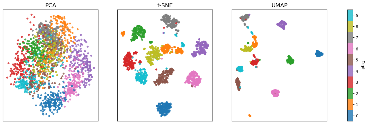
References
Healy, John, and Leland McInnes. 2024. “Uniform Manifold Approximation and Projection.” Nature Reviews Methods Primers 4 (1): 82.
Van der Maaten, Laurens, and Geoffrey Hinton. 2008. “Visualizing Data Using t-SNE.” Journal of Machine Learning Research 9 (11).