3.2.1. Diffusion Posterior Sampling (DPS)

Diffusion Posterior Sampling (DPS) (Chung et al. 2023) is a method for sampling from the posterior distribution in an inverse problem. To estimate the intractable likelihood term \(p_t(\boldsymbol{y} \mid \boldsymbol{x}_t)\), with \(\boldsymbol x \in \mathbb R^n\) and \(\boldsymbol y \in \mathbb R^m\) DPS first factored the distribution by marginalizing over the clean data \(\boldsymbol{x}_0\): \[ p_t(\boldsymbol{y} \mid \boldsymbol{x}_t) = \int p(\boldsymbol{y} \mid \boldsymbol{x}_0) p_t(\boldsymbol{x}_0 \mid \boldsymbol{x}_t) d\boldsymbol{x}_0 = \mathbb{E}_{\boldsymbol{x}_0 \sim p_t(\boldsymbol{x}_0 \mid \boldsymbol{x}_t)} \left[ p(\boldsymbol{y} \mid \boldsymbol{x}_0) \right]. \tag{1}\] This indicates that the likelihood of observing \(\boldsymbol{y}\) given a noisy image \(\boldsymbol{x}_t\) is the expected value of the clean data likelihood, weighted by the posterior \(p_t(\boldsymbol{x}_0 \mid \boldsymbol{x}_t)\). Because evaluating this expectation directly is intractable in practice, DPS proposed approximating it using the likelihood of the expected clean image: \[ p_t(\boldsymbol{y} \mid \boldsymbol{x}_t) \simeq p(\boldsymbol{y} \mid \boldsymbol{\hat{x}}_0), \tag{2}\] where \(\boldsymbol{\hat{x}}_0 \in \mathbb R^n\) is the posterior mean estimator computed via Tweedie’s formula: \[ \boldsymbol{\hat{x}}_0 = \mathbb{E}[\boldsymbol{x}_0 \mid \boldsymbol{x}_t] = \frac{1}{\sqrt{\overline{\alpha}_t}} \left( \boldsymbol{x}_t + (1 - \overline{\alpha}_t) \boldsymbol{s}_{\boldsymbol{\theta}} (\boldsymbol{x}_t, t) \right), \tag{3}\] where \(\overline{\alpha} \in \mathbb R\) is a parameter from the noise schedule.

Geometrically, while the score function \(\boldsymbol{s}_{\boldsymbol{\theta}} \in \mathbb R^n\) points in the direction orthogonal to the data manifold, the gradient of the likelihood term points in the tangent direction of the manifold. The specific form of the likelihood depends on the distribution of the measurement noise \(\boldsymbol{\epsilon}\), but it can be written in general as: \[ \nabla_{\boldsymbol{x}_t} \log p_t(\boldsymbol{y} \mid \boldsymbol{x}_t) \simeq - \rho \nabla_{\boldsymbol{x}_t} \left\| \boldsymbol{y} - \mathcal{A}(\boldsymbol{\hat{x}}_0) \right\|, \tag{4}\] where \(\|\cdot, \cdot\| : \mathbb R^{m\times m} \to \mathbb R_{\ge 0}\) is a norm and \(\rho \in \mathbb R\) is a step size.

Code

Importing the packages.

import torch
import deepinv as dinv
from torchvision import datasets, transforms
from diffusers import DDPMPipeline
import matplotlib.pyplot as plt

device = torch.device("cuda" if torch.cuda.is_available() else "cpu")

Creating an inpainting problem.

transform = transforms.Compose([
    transforms.ToTensor(),
    transforms.Normalize((0.5,), (0.5,))
])
mnist = datasets.MNIST(root='./data', train=False, download=True, transform=transform)

x_true = mnist[0][0].unsqueeze(0).to(device)

sigma = 0.001
physics = dinv.physics.Inpainting(
    mask=0.5,
    img_size=x_true.shape[1:],
    noise_model=dinv.physics.GaussianNoise(sigma=sigma),
    device=device,
)

y = physics(x_true)

dinv.utils.plotting.plot([x_true, y], titles=["Signal", "Measurement"])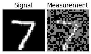

Loading a pre-trained MNIST Diffusion Model.

pipeline = DDPMPipeline.from_pretrained("1aurent/ddpm-mnist").to(device)
unet = pipeline.unet
scheduler = pipeline.scheduler
scheduler.set_timesteps(1000)
alphas_cumprod = scheduler.alphas_cumprod.to(device)

Reconstructing the image using DPS.

rho = 0.005
data_fidelity = dinv.optim.data_fidelity.L1()

x_t = torch.randn_like(x_true)

for i, t in enumerate(scheduler.timesteps):
    x_t = x_t.requires_grad_(True)
    noise_pred = unet(x_t, t).sample

    alpha_bar = alphas_cumprod[t]
    x_hat_0 = (x_t - (1 - alpha_bar).sqrt() * noise_pred) / alpha_bar.sqrt()

    loss = data_fidelity(x_hat_0, y, physics)

    grad = torch.autograd.grad(outputs=loss, inputs=x_t)[0]

    with torch.no_grad():
        prev_sample = scheduler.step(noise_pred, t, x_t).prev_sample

    x_t = (prev_sample - rho * grad).detach()

x_recon = x_t

Plotting the results.

imgs = [x_true, y, x_recon]
titles = [r"$\mathbf{x}_0$", r"$\mathbf{y}$", r"DPS Reconstruction"]

dinv.utils.plotting.plot(imgs, titles=titles, cmap="gray")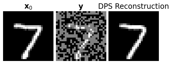

Source: dps.ipynb

References

Chung, Hyungjin, Jeongsol Kim, Michael T McCann, Marc L Klasky, and Jong Chul Ye. 2023. “Diffusion Posterior Sampling for General Noisy Inverse Problems.” In International Conference on Learning Representations.