2.4. Probabilistic Models

Probabilistic models treat the relationship between features \(\boldsymbol{x}\) and targets \(y\) as a result of stochastic processes. These models allow to quantify the uncertainty associated with the predictions – an important aspect in interpreting the model and decision-making.

Naive Bayes

Naive Bayes (NB) (Hand and Yu 2001) is a supervised learning algorithm based on applying Bayes’ theorem with the “naive” assumption of conditional independence between every pair of features given the value of the class variable. For a target class \(y\) and a feature vector \(\boldsymbol{x} \in \mathbb R^n\), Bayes’ theorem states: \[ P(y \mid \boldsymbol{x}) = \frac{P(\boldsymbol{x} \mid y) P(y)}{P(\boldsymbol{x})}. \tag{1}\] The “naive” assumption implies that: \[ P(x_i \mid y, x_1, \dots, x_{i-1}, x_{i+1}, \dots, x_n) = P(x_i \mid y), \tag{2}\] which simplifies the joint probability to a product of individual conditional probabilities: \[ P(y \mid \boldsymbol{x}) \propto P(y) \prod_{i=1}^{n} P(x_i \mid y). \tag{3}\] During inference, the predicted class \(\hat{y}\) is chosen by maximizing this posterior probability: \[ \hat{y} = \underset{y}{\arg \max} \ P(y) \prod_{i=1}^{n} P(x_i \mid y). \tag{4}\]

In general, NB is used as a classification baseline – as it makes “naive” assumptions about the relations between features and targets.

Code: Naive Bayes

Importing libraries for the NB.

import numpy as np
import matplotlib.pyplot as plt
from sklearn.datasets import make_blobs
from sklearn.naive_bayes import GaussianNB
from matplotlib.colors import ListedColormap
from sklearn.metrics import classification_report

Creating a synthetic dataset.

X, y = make_blobs(n_samples=300, centers=3, n_features=2, cluster_std=5.0, random_state=42)

Training the model.

gnb = GaussianNB()
gnb.fit(X, y)

GaussianNB()

In a Jupyter environment, please rerun this cell to show the HTML representation or trust the notebook.
On GitHub, the HTML representation is unable to render, please try loading this page with nbviewer.org.

Printing the decision boundaries of the model.

h = .02
x_min, x_max = X[:, 0].min() - 1, X[:, 0].max() + 1
y_min, y_max = X[:, 1].min() - 1, X[:, 1].max() + 1
xx, yy = np.meshgrid(np.arange(x_min, x_max, h), np.arange(y_min, y_max, h))

Z = gnb.predict(np.c_[xx.ravel(), yy.ravel()])
Z = Z.reshape(xx.shape)

plt.figure(figsize=(10, 6))
plt.contourf(xx, yy, Z, alpha=0.3, cmap='viridis')
plt.scatter(X[:, 0], X[:, 1], c=y, edgecolors='k', cmap='viridis')
plt.xlabel(r"$x_1$")
plt.ylabel(r"$x_2$")
plt.show()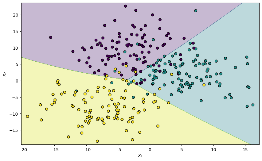

Source: nb.ipynb

Gaussian Processes (GPs)

Gaussian Processes (GPs) (Rasmussen 2003) extend the idea of probabilistic modeling to regression by defining a distribution over functions. While a standard regression model learns parameters of a specific function, a GP describes a distribution where any finite collection of function values has a joint Gaussian distribution.

A GP is specified by two components: its mean function \(\mu: \mathbb{R}^n \to \mathbb{R}\) and its kernel function \(k: \mathbb{R}^n \times \mathbb{R}^n \to \mathbb{R}\). The mean function provides the expected value at any point in the feature space, while the kernel function determines how to calculate the covariance between two observations. Together, they define the GP: \[ f(\boldsymbol{x}) \sim \mathcal{GP}\left(\mu(\boldsymbol{x}), k(\boldsymbol{x}, \boldsymbol{x}')\right). \tag{5}\] The kernel function \(k(\boldsymbol{x}, \boldsymbol{x}')\) encodes the prior assumptions about the properties of the function, such as smoothness and periodicity. Similar to the kernels used in Distance and Margin Models, the Radial Basis Function (RBF) is a common choice. As GPs are non-parametrical, the training only involves tuning the hyperparameters of the model.

During inference, given a training set \(\mathcal{D}^{(\text{Train})} = \{(\boldsymbol{x}_i^{(\text{Train})}, y_i^{(\text{Train})})\}_{i=1}^N\), the GP utilizes the joint distribution of the training data and a new test data point \(\boldsymbol{x}^{(\text{Test})}\) to calculate the posterior distribution \(P(f_* \mid \boldsymbol{x}^{(\text{Test})}, \mathcal{D}^{(\text{Train})})\). This results in a predictive mean \(\mu_*\), which serves as the point prediction, and a predictive variance \(\sigma_*^2\), which quantifies the model’s uncertainty: \[ \mu_* = \boldsymbol{k}_*^T \boldsymbol{K}^{-1} \boldsymbol{y}^{(\text{Train})}, \tag{6}\] \[ \sigma_*^2 = k(\boldsymbol{x}^{(\text{Test})}, \boldsymbol{x}^{(\text{Test})}) - \boldsymbol{k}_*^T \boldsymbol{K}^{-1} \boldsymbol{k}_*, \tag{7}\] where \(\boldsymbol{y}^{(\text{Train})} \in \mathbb R^N\) is the vector of training targets, \(\boldsymbol{K} \in \mathbb R^{N \times N}\) is the covariance matrix of the training data with entries \(\boldsymbol{K}_{i,j} = k(\boldsymbol{x}_i^{(\text{Train})}, \boldsymbol{x}_j^{(\text{Train})})\), and \(\boldsymbol{k}_* \in \mathbb R^N\) is the vector of covariances between the training data and the test point, where its \(i\)-th element is \(k(\boldsymbol{x}_i^{(\text{Train})}, \boldsymbol{x}^{(\text{Test})})\).

With that, GPs provide a mean curve and a confidence interval around it. This is specially useful for interpreting the uncertainty of the predictions, as well as potentially new regions to collected new data.

Code: Gaussian Processes

Importing libraries for the GP.

import numpy as np
import matplotlib.pyplot as plt
from sklearn.gaussian_process import GaussianProcessRegressor
from sklearn.gaussian_process.kernels import RBF, ConstantKernel as C

Creating a function and drawing noisy observations from it.

def f(x):
    return x * np.sin(x)

X = np.atleast_2d([1., 2.5, 3., 5., 6., 7., 8.]).T
y = f(X).ravel() + np.random.normal(0, 0.5, X.shape[0])

Training the model.

kernel = C(1.0, (1e-3, 1e3)) * RBF(10, (1e-2, 1e2))
gp = GaussianProcessRegressor(kernel=kernel, n_restarts_optimizer=9, alpha=0.1)
gp.fit(X, y)

GaussianProcessRegressor(alpha=0.1, kernel=1**2 * RBF(length_scale=10),
                         n_restarts_optimizer=9)

Plotting the prediction.

x_range = np.atleast_2d(np.linspace(0, 10, 1000)).T
y_pred, sigma = gp.predict(x_range, return_std=True)

plt.figure(figsize=(10, 6))
plt.plot(x_range, f(x_range), 'r:', label=r'$f(x) = x \sin(x)$')
plt.plot(X, y, 'r.', markersize=10, label='Observations')
plt.plot(x_range, y_pred, 'b-', label='GP Mean')
plt.fill_between(x_range.ravel(), y_pred - 1.96 * sigma, y_pred + 1.96 * sigma,
                 alpha=0.2, color='blue', label='GP 95% Confidence Interval')

plt.xlabel('$x$')
plt.ylabel('$f(x)$')
plt.legend(loc='upper left')
plt.show()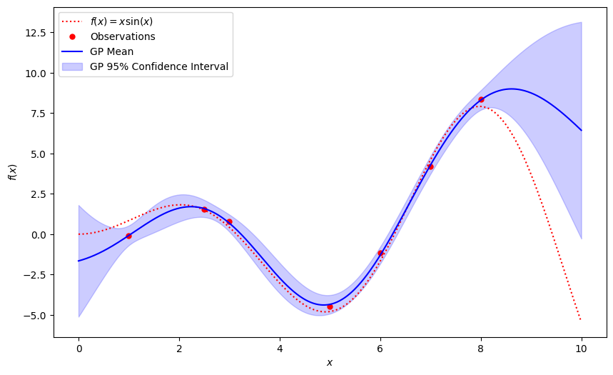

Source: gp.ipynb

References

Hand, David J, and Keming Yu. 2001. “Idiot’s Bayes—Not so Stupid After All?” International Statistical Review 69 (3): 385–98.

Rasmussen, Carl Edward. 2003. “Gaussian Processes in Machine Learning.” In Summer School on Machine Learning, 63–71. Springer.