1.1.1. Score Matching with Langevin Dynamics (SMLD)

Score Matching with Langevin Dynamics (SMLD) (Song and Ermon 2019) was the first formulation of the current Diffusion Models (DMs). The idea was to approximate the score function of the data distribution to generate new images. Therefore, given a data distribution \(p(\boldsymbol{x}_0)\) with \(\boldsymbol x_0 \in \mathbb R^n\), the goal was to approximate the score function \(\nabla_{\boldsymbol{x}_0} \log p(\boldsymbol{x}_0): \mathbb R^n \to \mathbb R^n\) with a Neural Network (NN) \(\boldsymbol{s}_{\boldsymbol{\theta}} : \mathbb R^n \to \mathbb R^n\). The reason is that the score function indicates regions in space with higher data density, therefore, approximating this term helps to reach regions in space where the dataset lies.

Although this could be done using a mean squared error approach, the score function only has relevant signal in regions of high data density. Therefore, a denoising approach was used to overcome the fact that real data typically resides on a low-dimensional manifold embedded in a high-dimensional space. In the empty spaces between valid data points, the probability density \(p(\boldsymbol{x}_0) \approx 0\), which makes the score function contain close to no information.

To solve this, SMLD corrupted the data with a sequence of Gaussian noise scales, \(\sigma_T > \sigma_{T-1} > \dots > \sigma_1\), where \(\sigma_t \in \mathbb R^{+}\). The largest noise scale was chosen to be large enough to provide relevant signal across the entire space, while the smallest scale was chosen to be small enough to approximate the clean data distribution. The NN \(\boldsymbol{s}_{\boldsymbol{\theta}}(\boldsymbol{x}_t, \sigma_t) : \mathbb R^{n\times 1} \to \mathbb R^n\) was then trained to predict the score across all the noise levels. For a specific noise scale \(\sigma_t\), the perturbation kernel is Gaussian, being given by: \[ q_{\sigma_t}(\boldsymbol{x}_t \mid \boldsymbol{x}_0) = \mathcal{N}(\boldsymbol{x}_t \mid \boldsymbol{x}_0, \sigma_t^2 \boldsymbol{I}), \tag{1}\] which yields a score of \(\nabla_{\boldsymbol{x}_t} \log q_{\sigma_t}(\boldsymbol{x}_t \mid \boldsymbol{x}_0) = - \frac{\boldsymbol{x}_t - \boldsymbol{x}_0}{\sigma_t^2}\). Therefore, the loss function was defined as: \[ \mathcal{L}(\boldsymbol{\theta}) = \mathbb{E}_{\boldsymbol{x}_0, \boldsymbol{x}_t, t} \left[ \lambda(t) \mathcal{L}_{\sigma_t}(\boldsymbol{\theta}) \right], \tag{2}\] where \(\lambda(t) = \sigma_t^2\) is a weighting function and \[ \mathcal{L}_{\sigma_t}(\boldsymbol{\theta}) = \frac{1}{2} \mathbb{E}_{\boldsymbol{x}_0, \boldsymbol{x}_t} \left[ \left\| \boldsymbol{s}_{\boldsymbol{\theta}}(\boldsymbol{x}_t, \sigma_t) + \frac{\boldsymbol{x}_t - \boldsymbol{x}_0}{\sigma_t^2} \right\|_2^2 \right]. \tag{3}\]

To synthesize new data, SMLD employed the Annealed Langevin Dynamics method.

Code

Importing the packages.

import torch
import numpy as np
import matplotlib.pyplot as plt
from torchvision import transforms
from torchvision.datasets import MNIST

Plotting the noise schedule of SMLD.

T = 100
sigma_1 = 0.01
sigma_T = 10.0

steps = np.arange(1, T + 1)
smld_sigmas = sigma_1 * ((sigma_T / sigma_1) ** ((steps - 1) / (T - 1)))

plt.figure(figsize=(10, 4))
plt.plot(steps, smld_sigmas, color="blue", linewidth=2.5)
plt.xlabel(r"$t$", fontsize=12)
plt.ylabel(r"$\sigma_t$", fontsize=12)
plt.grid(True, which="both", linestyle="--", alpha=0.5)
plt.tight_layout()
plt.show()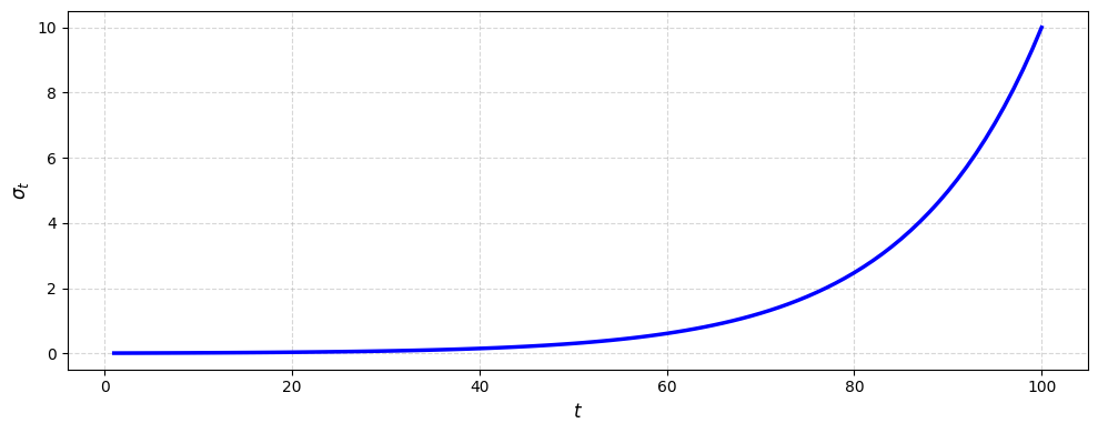

Showing the data corruption in different noise scales.

dataset = MNIST(root="./data", train=True, download=True, transform=transforms.ToTensor())
x0, _ = dataset[0]
x0 = x0.unsqueeze(0)

selected_indices = [0, 15, 35, 55, 75, 99]
fig, axes = plt.subplots(1, len(selected_indices) + 1, figsize=(16, 3))

axes[0].imshow(x0.squeeze().numpy(), cmap="gray")
axes[0].set_title(r"Original $\mathbf{x}_0$", fontsize=12)
axes[0].axis("off")

for i, idx in enumerate(selected_indices):
    sigma = smld_sigmas[idx]
    z = torch.randn_like(x0)
    xt = x0 + sigma * z

    axes[i + 1].imshow(xt.squeeze().numpy(), cmap="gray")
    axes[i + 1].set_title(r"$\sigma_t=$" + f"{sigma:.2f}", fontsize=11)
    axes[i + 1].axis("off")

plt.tight_layout()
plt.show()

Source: smld.ipynb

References

Song, Yang, and Stefano Ermon. 2019. “Generative Modeling by Estimating Gradients of the Data Distribution.” Advances in Neural Information Processing Systems 32.