import numpy as np
import matplotlib.pyplot as plt
from sklearn.ensemble import IsolationForest
from sklearn.neighbors import LocalOutlierFactor3.3. Outlier Identification
Identifying outliers involves searching for observations that do not fit the patterns of the rest of the data. Outliers are not necessarily errors or values that should be ignored or excluded, they are unusual observations that should be examined with caution. Models such as linear regression are highly sensitive to outliers, thus identifying these points serves as a warning for further study of the dataset.
Local Outlier Factor (LOF)
The Local Outlier Factor (LOF) (Breunig et al. 2000) algorithm uses the density of neighbors of a point to determine whether it is an outlier. Firstly, the hyperparameter \(k\) is defined, representing the number of neighbors considered. Given a point \(\boldsymbol{x}\), \(\eta_k(\boldsymbol{x})\) denotes the set of the \(k\) nearest neighbors, and \(d_k(\boldsymbol{x})\) denotes the distance from \(\boldsymbol{x}\) to its \(k\)-th nearest neighbor. Note that \(\eta_k(\boldsymbol{x})\) can contain more than \(k\) elements in the case of a tie. The reachability distance \(D_k(\boldsymbol{x}_i, \boldsymbol{x}_j)\) is then defined as: \[ D_k(\boldsymbol{x}_i, \boldsymbol{x}_j) = \max\{d_k(\boldsymbol{x}_j), d(\boldsymbol{x}_i, \boldsymbol{x}_j)\}. \tag{1}\] In words, the distance \(D_k\) is the distance from \(\boldsymbol{x}_i\) to \(\boldsymbol{x}_j\), but never less than \(d_k(\boldsymbol{x}_j)\). As it is not symmetric, this function is not a true mathematical distance. Next, the local reachability density \(L_k(\boldsymbol{x}_i)\) of \(\boldsymbol{x}_i\) is defined as: \[ L_k(\boldsymbol{x}_i) = \left(\frac{1}{|\eta_k(\boldsymbol{x}_i)|}\sum\limits_{\boldsymbol{x}_j \in \eta_k(\boldsymbol{x}_i)} D_k(\boldsymbol{x}_i,\boldsymbol{x}_j)\right)^{-1}. \tag{2}\] This corresponds to the inverse of the average reachability distance of \(\boldsymbol{x}_i\) from its neighbors. Finally, the LOF value for a point \(\boldsymbol{x}_i\) is given by: \[ \text{LOF}_k(\boldsymbol{x}_i) = \frac{1}{|\eta_k(\boldsymbol{x}_i)|} \sum\limits_{\boldsymbol{x}_j \in \eta_k(\boldsymbol{x}_i)} \frac{L_k(\boldsymbol{x}_j)}{L_k(\boldsymbol{x}_i)}. \tag{3}\] The expression above divides the average distance at which its neighbors can be reached with the average distance at which the point can be accessed. Therefore, values close to \(1\) shows that the point \(\boldsymbol{x}_i\) is not an outlier, values much lower than \(1\) present an inlier, and values much bigger than \(1\) represent outliers.
Isolation Forest (IF)
Isolation Forest (IF) (Liu, Ting, and Zhou 2008) works similarly to Random Forest. The intuition behind this algorithm is that outliers are more easily isolated than the rest of the data. Each tree randomly selects a feature at each split and, within the range of values of that feature, performs a separation. This process is repeated until all data points are isolated in leaf nodes. The average depth at which the data points are isolated is then computed. Points with shorter average path lengths are more likely to be outliers. Based on a threshold, each point is classified as either an outlier or an inlier.
Code
Importing the packages.
Creating a synthetic dataset.
np.random.seed(42)
X_inliers = 0.3 * np.random.randn(100, 2)
X_inliers = np.r_[X_inliers + 2, X_inliers - 2]
X_outliers = np.random.uniform(low=-4, high=4, size=(20, 2))
X = np.r_[X_inliers, X_outliers]
Instantiating and fitting the methods.
iso_forest = IsolationForest(contamination=0.15, random_state=42)
y_pred_iso = iso_forest.fit_predict(X)

lof = LocalOutlierFactor(n_neighbors=20, contamination=0.15)
y_pred_lof = lof.fit_predict(X)
Plotting the results, where the red dots are outliers.
plt.figure(figsize=(14, 6))

plt.subplot(1, 2, 1)
plt.title("Isolation Forest")
colors_iso = np.array(['red' if label == -1 else 'blue' for label in y_pred_iso])
plt.scatter(X[:, 0], X[:, 1], c=colors_iso, edgecolor='k', alpha=0.7)
plt.xlabel("Feature 1")
plt.ylabel("Feature 2")

plt.subplot(1, 2, 2)
plt.title("Local Outlier Factor")
colors_lof = np.array(['red' if label == -1 else 'blue' for label in y_pred_lof])
plt.scatter(X[:, 0], X[:, 1], c=colors_lof, edgecolor='k', alpha=0.7)
plt.xlabel("Feature 1")
plt.ylabel("Feature 2")

plt.tight_layout()
plt.show()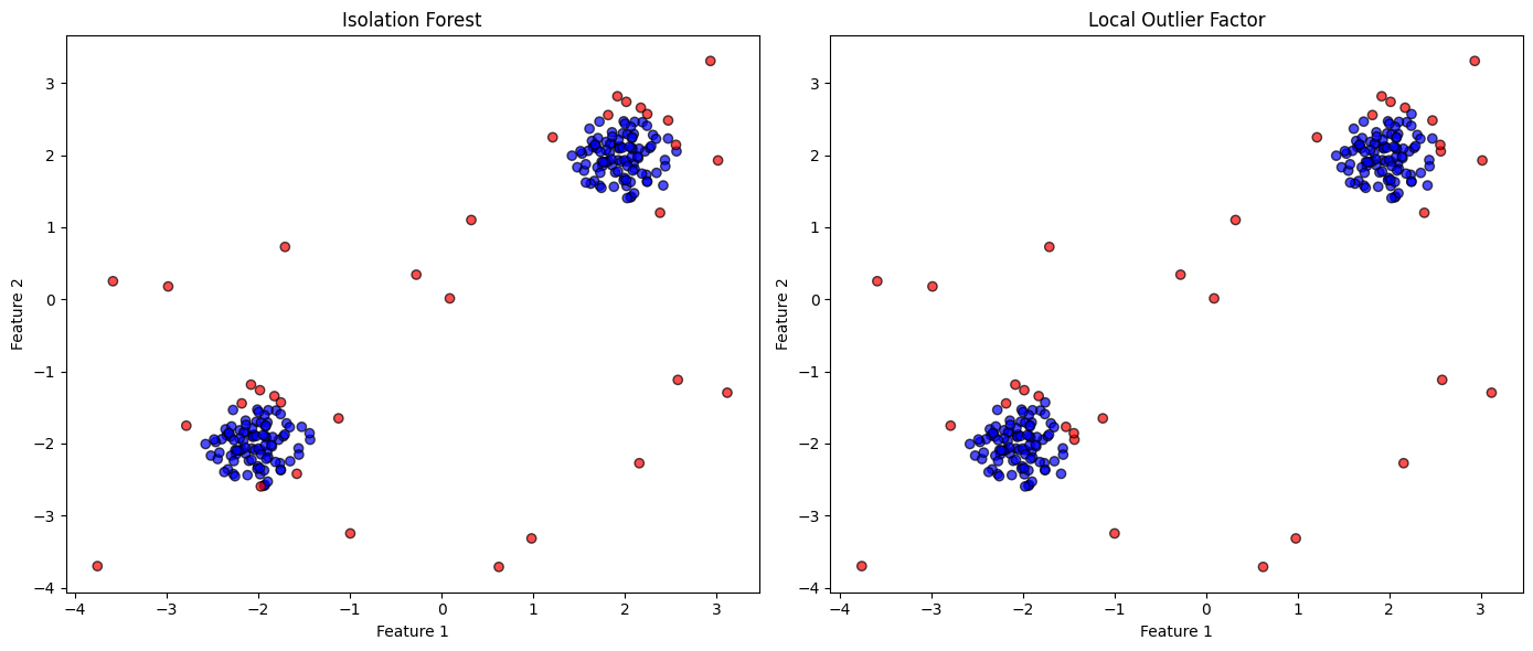
References
Breunig, Markus M, Hans-Peter Kriegel, Raymond T Ng, and Jörg Sander. 2000. “LOF: Identifying Density-Based Local Outliers.” In International Conference on Management of Data, 93–104.
Liu, Fei Tony, Kai Ming Ting, and Zhi-Hua Zhou. 2008. “Isolation Forest.” In International Conference on Data Mining, 413–22. IEEE.