1.1.4. Graph Diffusion via the System of SDEs (GDSS)

Following the Stochastic Differential Equations (SDEs) connection with generative diffusion, Graph Diffusion via the System of SDEs (GDSS) (Jo, Lee, and Hwang 2022) extended this approach to graph generation. The idea was to couple the diffusion of the adjacency and node features, creating a system of SDEs.

Let \(\boldsymbol G = (\boldsymbol X, \boldsymbol A) \in \mathbb R^{N\times d} \times \mathbb R^{N\times N}\) be a graph composed of a weighted adjacency matrix \(\boldsymbol A\) and \(N\) node features \(\boldsymbol X\) of dimension \(d\). To jointly diffuse the nodes and edges, the diffusion process is formulated by building a trajectory \(\{\boldsymbol G_t = (\boldsymbol X_t, \boldsymbol A_t)\}_{t\in [0, T]}\), where \(T\) is the end of the diffusion process. As previously established, this is modelled by the following SDE: \[ d\boldsymbol G = \boldsymbol f(\boldsymbol G, t) dt + g(t) \boldsymbol w, \tag{1}\] where \(\boldsymbol{w} \in \mathcal G\) is the Wiener process, \(\boldsymbol{f} : \mathcal G \times \mathbb R \to \mathbb R^\mathcal{G}\) is the drift coefficient and \(g : \mathbb R \to \mathbb R\) is the diffusion coefficient, with \(\mathcal G\) being the space where the graph is embedded. Given the forward process, the reverse time SDE is given by: \[ d\boldsymbol G = \left[\boldsymbol f(\boldsymbol G, t) - g(t)^2 \nabla_{\boldsymbol G} \log p_t(\boldsymbol G) \right] dt + g(t) \boldsymbol{\overline{w}}, \tag{2}\] where \(\boldsymbol{\overline w} \in \mathcal G\) is the Wiener process running from \(T\) to \(0\). Therefore, the goal is to approximate the score function in order to sample from the initial data distribution. The problem is that this function is expensive to compute, as the graph space is very high-dimensional. To overcome this issue, a system of reverse time SDEs was proposed, following: \[ \begin{cases} d\boldsymbol X = \left[\boldsymbol f_{\boldsymbol X}(\boldsymbol X, t) - g_{\boldsymbol X}(t)^2 \nabla_{\boldsymbol X} \log p_t(\boldsymbol X, \boldsymbol A) \right] dt + g_{\boldsymbol X}(t) \boldsymbol{\overline{w}_{\boldsymbol X}} \\ d\boldsymbol A = \left[\boldsymbol f_{\boldsymbol A}(\boldsymbol A, t) - g_{\boldsymbol A}(t)^2 \nabla_{\boldsymbol A} \log p_t(\boldsymbol X, \boldsymbol A) \right] dt + g_{\boldsymbol A}(t) \boldsymbol{\overline{w}_{\boldsymbol A}} \end{cases}, \tag{3}\] where \(\boldsymbol f(\boldsymbol G, t) = (\boldsymbol f_{\boldsymbol X} (\boldsymbol X), \boldsymbol f_{\boldsymbol A} (\boldsymbol A))\) are the drift components, \(g_{\boldsymbol X}\) and \(g_{\boldsymbol A}\) are the diffusion coefficients, and \(\boldsymbol{\overline{w}_{\boldsymbol X}}\) and \(\boldsymbol{\overline{w}_{\boldsymbol A}}\) are the respective Wiener processes running backwards in time. With that, each graph component was diffused separately, while their reverse time SDEs were coupled by the joint score function of the data distribution.

To approximate these partial score functions, GDSS employed Graph Neural Networks (GNNs) parameterized by \(\boldsymbol{\theta}\) and \(\boldsymbol \phi\). The GNNs received the noisy graph tuple \((\boldsymbol{X}_t, \boldsymbol{A}_t)\) at time \(t\), respectively approximating one of the partial score functions: \[ \boldsymbol{s}_{\boldsymbol{\theta}}(\boldsymbol{X}_t, \boldsymbol{A}_t, t) \approx \nabla_{\boldsymbol{X}} \log p_t(\boldsymbol{X}, \boldsymbol{A}) \quad \text{and} \quad \boldsymbol{s}_{\boldsymbol{\phi}}(\boldsymbol{X}_t, \boldsymbol{A}_t, t) \approx \nabla_{\boldsymbol{A}} \log p_t(\boldsymbol{X}, \boldsymbol{A}). \tag{4}\] By sharing the topological structure as input, the estimation of the node and edge scores remained coupled, even though the networks \(\boldsymbol{\theta}\) and \(\boldsymbol{\phi}\) were optimized independently.

The models were trained using a joint denoising score matching objective, which minimized: \[ \mathcal{L}(\boldsymbol{\theta}, \boldsymbol{\phi}) = \mathbb{E}_{t, \boldsymbol{G}_0, \boldsymbol{G}_t} \left[ \lambda_{\boldsymbol{X}}(t) \left\| \boldsymbol{s}_{\boldsymbol{\theta}} - \nabla_{\boldsymbol{X}_t} \log q_{0t}(\boldsymbol{X}_t \mid \boldsymbol{X}_0) \right\|_2^2 + \lambda_{\boldsymbol{A}}(t) \left\| \boldsymbol{s}_{\boldsymbol{\phi}} - \nabla_{\boldsymbol{A}_t} \log q_{0t}(\boldsymbol{A}_t \mid \boldsymbol{A}_0) \right\|_2^2 \right], \tag{5}\] where \(q_{0t}\) represents the perturbation kernel of the forward SDEs and \(\lambda_{\boldsymbol{X}}(t) : \mathbb R \to \mathbb R\) and \(\lambda_{\boldsymbol{A}}(t) : \mathbb R \to \mathbb R\) are positive weighting functions.

In order to sample from the model, a two-step procedure was employed. First, the size of the graph was sampled from the empirical distribution of graph sizes in the training data. Given \(N\), algorithms based on Predictor-Corrector (PC) were developed to sample from the system of revere time SDEs.

Code

Importing the packages.

import torch
import networkx as nx
import matplotlib.pyplot as plt

Creating a toy graph.

N = 10
d = 3
G = nx.cycle_graph(N)

A_0 = torch.tensor(nx.to_numpy_array(G), dtype=torch.float32)
X_0 = torch.ones((N, d), dtype=torch.float32)

Using a Variance Preserving SDE (VP-SDE) to corrupt the data.

T = 1000
betas = torch.linspace(1e-4, 0.02, T)
alphas = 1.0 - betas
alphas_cumprod = torch.cumprod(alphas, dim=0)

def corrupt_graph(A_0, X_0, t):
    alpha_bar = alphas_cumprod[t]

    noise_X = torch.randn_like(X_0)

    noise_A_raw = torch.randn_like(A_0)
    noise_A_upper = torch.triu(noise_A_raw, diagonal=1)
    noise_A = noise_A_upper + noise_A_upper.T

    X_t = torch.sqrt(alpha_bar) * X_0 + torch.sqrt(1 - alpha_bar) * noise_X
    A_t = torch.sqrt(alpha_bar) * A_0 + torch.sqrt(1 - alpha_bar) * noise_A

    return X_t, A_t

Simulating a forward process.

timesteps = [0, 100, 500, 999]
fig, axs = plt.subplots(2, len(timesteps), figsize=(15, 4))

for i, t in enumerate(timesteps):
    X_t, A_t = corrupt_graph(A_0, X_0, t)

    axs[0, i].imshow(A_t.numpy(), cmap='viridis', vmin=-1.5, vmax=1.5)
    axs[1, i].imshow(X_t.numpy(), cmap='viridis', vmin=-1.5, vmax=1.5)

    axs[0, i].set_title(f"t = {t}")
    axs[0, i].set_ylabel(r"$\boldsymbol{A}_t$")
    axs[1, i].set_ylabel(r"$\boldsymbol{X}_t$")

plt.show()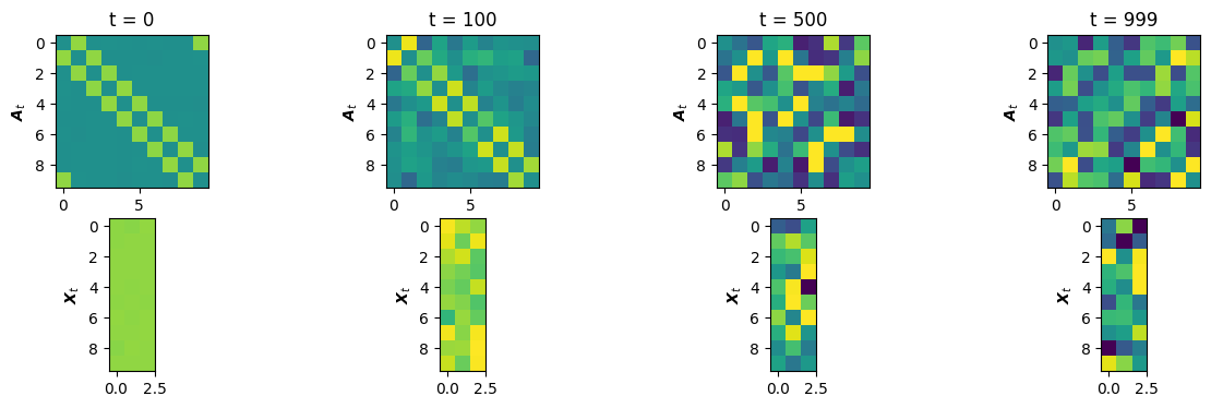

Source: gdss.ipynb

References

Jo, Jaehyeong, Seul Lee, and Sung Ju Hwang. 2022. “Score-Based Generative Modeling of Graphs via the System of Stochastic Differential Equations.” In International Conference on Machine Learning, 10362–83. PMLR.