import numpy as np
import pandas as pd
import matplotlib.pyplot as plt
from sklearn.datasets import fetch_california_housing
from sklearn.model_selection import train_test_split
from sklearn.ensemble import RandomForestRegressor

import shap
import lime
import lime.lime_tabular1.4. Model Explanation
Model explanation is a class of techniques that aim to explain models that are not interpretable, using indirect importance of the features. This is the last step of a Machine Leaning (ML) pipeline, where the user extracts useful information about the patterns of the trained models.
Local Interpretable Model-Agnostic Explanations (LIME)
One of these techniques is the Local Interpretable Model-agnostic Explanations (LIME) (Ribeiro, Singh, and Guestrin 2016). LIME locally approximates the original model \(f\) with an interpretable model \(g\in G\), where \(G\) is the class of interpretable models. The interpretable model receives an interpretable representation of the inputs, which is denoted by \(\boldsymbol x = h(\boldsymbol{x}')\), where \(h\) maps the original data into a binary representation in the space of features. For images, the interpretable representations could be super-pixels, such that a value of 1 in \(\boldsymbol{x}'\) represents the presence of that specific super-pixel.
To formulate the importance of each feature, some definitions are needed. Let \(\pi_{\boldsymbol{x}} (\boldsymbol{z})\) be a measure of proximity of \(\boldsymbol{z}\) to \(\boldsymbol{x}\), modeling its neighborhood. Let \(\mathcal L(f, g, \pi_{\boldsymbol{x}})\) be the measure of how different \(g\) approximates \(f\) is the locality defined by \(\pi_{\boldsymbol{x}}\). Finally, let \(\Omega(g)\) be a term involving the complexity of the model \(g\). The explanation of the LIME method is obtained minimizing the following equation: \[ \underset{g\in G}{\arg\min} \ \mathcal L(f, g, \pi_{\boldsymbol{x}}) + \Omega(g). \tag{1}\] The choice of \(g\) is usually a linear model, such as a linear regression, while the neighborhood is defined on a Gaussian kernel. The loss function is dependent on the data type and on the task being performed. The importance of the features is attributed to their importance on the interpretable model. Being a local explanation, LIME samples data according to the neighborhood defined on the algorithm. With that, explanations could be unstable, according to the parameters that define \(\pi_{\boldsymbol{x}}\).
SHapley Additive exPlanations (SHAP)
Shapely values were first introduced in Game Theory, as a way to split a certain reward to a set of players, following certain justice axioms (Lundberg and Lee 2017). To explain the Shapley values, let \(N\) be a set of players and \(S_i\) be the set of all subsets of \(N\) where the player \(i\) is not present, that is \(S\subseteq N\setminus\{i\}\). Then, the Shapley value of the \(i\)-th player is defined as: \[ \phi_i (f) = \sum_{S \in S_i} \frac{|S|! (|N| - |S| - 1)!}{|N|!}\big[ f(S \cup \{i\}) - f(S) \big], \tag{2}\] where \(|\cdot|\) denotes the cardinality of a set, and \(f(\cdot)\) is a function that returns the contribution of a given coalition. Note that this definition does not take the order of players into account, though it is possible to add this information.
The Shapley values obey certain axioms that define a fair payout. The first one is the efficiency axiom, where it is stated that the sum of all players’ contributions must equal the total prize. \[ \sum_{i=1}^N \phi_i = f(N) - f(\emptyset). \tag{3}\] The next axioms ensure a fair distribution of the prize. The symmetry axiom states that if two players contribute equally to all possible coalitions, their Shapley values must be identical. With that \[ f(S \cup \{i\}) = f(S \cup \{j\}), \ \forall S \subseteq N\setminus\{i, j\} \Rightarrow \phi_i(f) = \phi_j(f). \tag{4}\] Next, the dummy player axiom states that a player that does not change the outcome of any coalition has a Shapley value of zero, that is: \[ f(S \cup \{i\}) = f(S), \ \forall \subseteq N\setminus\{i\}\Rightarrow \phi_i(f) = 0. \tag{5}\] Finally, the Shapley values follow the additivity property. In a game composed of two separate games \(f+w\), the Shapley value for a player is the sum of their individual Shapley values in each game: \[ \phi_i(f+w) = \phi_i(f) + \phi_i(w). \tag{6}\] It was proven that the only way to distribute the final prize into the set of players, following the previous axioms, is by the Shapley values definition.
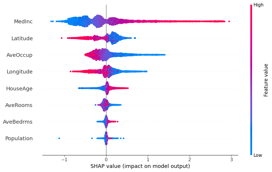
In the context of ML model explanation, SHAP (SHapley Additive exPlanations) adapts this concept by treating features as players in a game. The game is the task of predicting the output for a specific instance, while the prize is the difference between the model’s prediction for that instance and the base value. The function \(f(S)\) represents the expected output of the model given only the set of features \(S\). SHAP introduced a new class of additive feature attribution methods, where an explanation is represented as a linear model: \[ g(\boldsymbol{z}') = \phi_0 + \sum_{i=1}^{n} \phi_i z'_i, \tag{7}\] where \(g\) is the explanation model, \(\boldsymbol{z}' \in \{0, 1\}^n\) is a simplified binary representation indicating the presence or absence of a feature, \(n\) is the number of features, and \(\phi_i\) is the feature attribution for feature \(i\), which is its Shapley value. The term \(\phi_0\) represents the base value, that is, \(\mathbb E[f(\boldsymbol{x})]\). A significant challenge is that the exact computation of Shapley values is computationally expensive, as it requires evaluating the model for all \(2^n\) possible feature subsets. In order to solve this problem, the original work of SHAP introduced various alternatives to solve this.
Code
Importing the packages.
Loading the dataset with California houses’s prices.
data = fetch_california_housing()
X = pd.DataFrame(data.data, columns=data.feature_names)
y = data.target

X_train, X_test, y_train, y_test = train_test_split(X, y, test_size=0.2, random_state=42)
Training a Random Forest.
model = RandomForestRegressor(n_estimators=100, max_depth=12, random_state=42)
model.fit(X_train, y_train)
RandomForestRegressor(max_depth=12, random_state=42)In a Jupyter environment, please rerun this cell to show the HTML representation or trust the notebook.
On GitHub, the HTML representation is unable to render, please try loading this page with nbviewer.org.
RandomForestRegressor(max_depth=12, random_state=42)
Choosing a test sample for local explainability.
sample_idx = 0
instance = X_test.iloc[[sample_idx]]
print(instance.T)
print(f"True Target Value: {y_test[sample_idx]:.4f}")
print(f"Model Prediction: {model.predict(instance)[0]:.4f}")
20046
MedInc 1.681200
HouseAge 25.000000
AveRooms 4.192201
AveBedrms 1.022284
Population 1392.000000
AveOccup 3.877437
Latitude 36.060000
Longitude -119.010000
True Target Value: 0.4770
Model Prediction: 0.5416Calculating the SHAP values and plotting the local and global importance of the features.
explainer_shap = shap.TreeExplainer(model)
shap_values = explainer_shap(X_test)

plt.figure(figsize=(10, 6))
shap.plots.waterfall(shap_values[sample_idx], show=False)
plt.gcf().set_size_inches(10, 5)
plt.tight_layout()
plt.show()

plt.figure(figsize=(10, 6))
shap.plots.beeswarm(shap_values, show=False)
plt.gcf().set_size_inches(10, 6)
plt.tight_layout()
plt.show()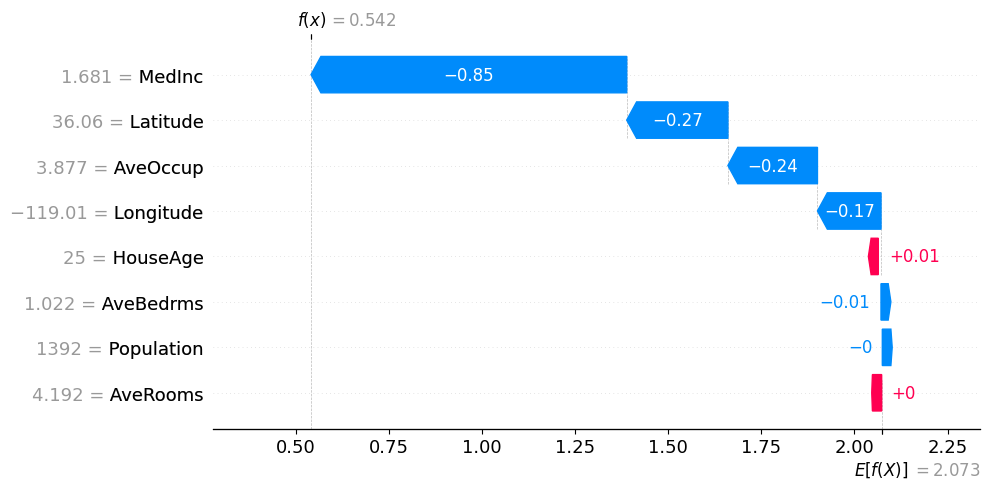
Doing the same for LIME values, plotting the local importance of the features.
explainer_lime = lime.lime_tabular.LimeTabularExplainer(
    training_data=np.array(X_train),
    feature_names=X_train.columns,
    class_names=['MedHouseValue'],
    mode='regression',
    random_state=42
)

exp = explainer_lime.explain_instance(
    data_row=X_test.iloc[sample_idx],
    predict_fn=model.predict,
    num_features=5
)

plt.figure(figsize=(10, 5))
exp.as_pyplot_figure()
plt.tight_layout()
plt.show()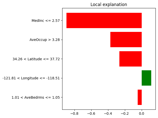
References
Lundberg, Scott M, and Su-In Lee. 2017. “A Unified Approach to Interpreting Model Predictions.” Advances in Neural Information Processing Systems 30.
Ribeiro, Marco Tulio, Sameer Singh, and Carlos Guestrin. 2016. “‘Why Should i Trust You?’ Explaining the Predictions of Any Classifier.” In International Conference on Knowledge Discovery and Data Mining, 1135–44.