import numpy as np
import matplotlib.pyplot as plt
from sklearn.datasets import make_blobs, make_moons, make_circles
from sklearn.cluster import KMeans, DBSCAN, AgglomerativeClustering3.2. Clustering
One of the primary tasks of Unsupervised Learning is to group similar data observations based on their features. This process is known as clustering. While clustering algorithms share structural similarities with Supervised Learning methods, they operate on unlabeled datasets.
\(k\)-Means
The \(k\)-Means (McQueen 1967) clustering algorithm is similar to the supervised \(k\)-NN model, but here, the hyperparameter \(k\) dictates the number of clusters rather than neighbors.
The algorithm initializes by selecting \(k\) random data points to act as initial cluster centers, or centroids. Using a defined distance metric, the distance from each data point to every centroid is calculated. Each observation is then assigned to the cluster of its nearest centroid. Subsequently, each centroid \(\boldsymbol{c}_j\) is updated by calculating the mean of all points assigned to its cluster \(\mathcal{C}_j\): \[ \boldsymbol{c}_j = \frac{1}{|\mathcal{C}_j|} \sum_{\boldsymbol{x}_i \in \mathcal{C}_j} \boldsymbol{x}_i, \tag{1}\] where \(|\mathcal{C}_j|\) denotes the number of observations in cluster \(j\). This process is repeated until the centroids converge and the cluster assignments no longer change. Because the parameter \(k\) is predefined, it is typically identified using validation metrics.
Density-Based Spatial Clustering of Applications with Noise (DBSCAN)
Density-Based Spatial Clustering of Applications with Noise (DBSCAN) (Ester et al. 1996) identifies clusters based on the local density of points in the feature space. The algorithm relies on two hyperparameters: \(\epsilon > 0\), defining the search radius of the neighborhood, and \(M > 0\), the minimum number of points required within that radius to constitute a dense region.
Based on these thresholds, the algorithm classifies each data point into one of three categories:
- Core Point: an observation with at least \(M\) neighbors within its \(\epsilon\)-radius;
- Border Point: an observation with fewer than \(M\) neighbors within \(\epsilon\), but that falls within the neighborhood of a core point;
- Noise Point: an observation that meets neither condition.
The algorithm forms clusters by connecting adjacent core points and their respective border points. Noise points are left unassigned. Unlike \(k\)-Means, DBSCAN does not require specifying the number of clusters a priori and can discover clusters of arbitrary shapes, though it can struggle with datasets containing different local densities.
Hierarchical Clustering
Hierarchical clustering algorithms construct a tree-like structure of clusters and are typically formulated using one of two strategies: agglomerative or divisive. The agglomerative strategy initializes with each data point representing its own singleton cluster, iteratively merging the closest pairs. The divisive strategy starts with all points in a single cluster, recursively splitting them.
In an agglomerative framework, the algorithm computes a distance matrix for all clusters and merges the two closest clusters at each iteration. The definition of “closest” depends on the chosen linkage criterion. The algorithm terminates either when a single unified cluster remains or when the distance between merging clusters exceeds a predefined arbitrary threshold. After finished, a hierarchical structure can be observed in the formation of the clusters.
Code
Importing the packages.
Creating distinct synthetic datasets.
n_samples = 300
random_state = 42

X_blobs, _ = make_blobs(n_samples=n_samples, centers=3, cluster_std=0.6, random_state=random_state)
X_moons, _ = make_moons(n_samples=n_samples, noise=0.05, random_state=random_state)
X_circles, _ = make_circles(n_samples=n_samples, factor=0.5, noise=0.05, random_state=random_state)

datasets = [
    ("Globular Data", X_blobs),
    ("Arbitrary Shapes", X_moons),
    ("Concentric Geometry", X_circles)
]
Instantiating the methods.
models = [
    ("k-Means", KMeans(n_clusters=3, random_state=random_state, n_init=10)),
    ("DBSCAN", DBSCAN(eps=0.2, min_samples=5)),
    ("Agglomerative (Single Linkage)", AgglomerativeClustering(n_clusters=2, linkage='single'))
]
Fitting and plotting the results.
fig, axes = plt.subplots(len(datasets), len(models), figsize=(15, 12))
plt.subplots_adjust(hspace=0.3, wspace=0.1)

for row_idx, (data_name, X) in enumerate(datasets):
    for col_idx, (model_name, model) in enumerate(models):
        ax = axes[row_idx, col_idx]

        y_pred = model.fit_predict(X)

        clustered_mask = y_pred != -1
        ax.scatter(X[clustered_mask, 0], X[clustered_mask, 1],
                   c=y_pred[clustered_mask], cmap='viridis',
                   s=30, edgecolor='k')

        noise_mask = y_pred == -1
        if np.any(noise_mask):
            ax.scatter(X[noise_mask, 0], X[noise_mask, 1],
                       c='black',
                       s=30, edgecolor='k', alpha=0.8)

        ax.set_xticks([])
        ax.set_yticks([])

        if row_idx == 0:
            ax.set_title(model_name, fontsize=14)

        if col_idx == 0:
            ax.set_ylabel(data_name, fontsize=14)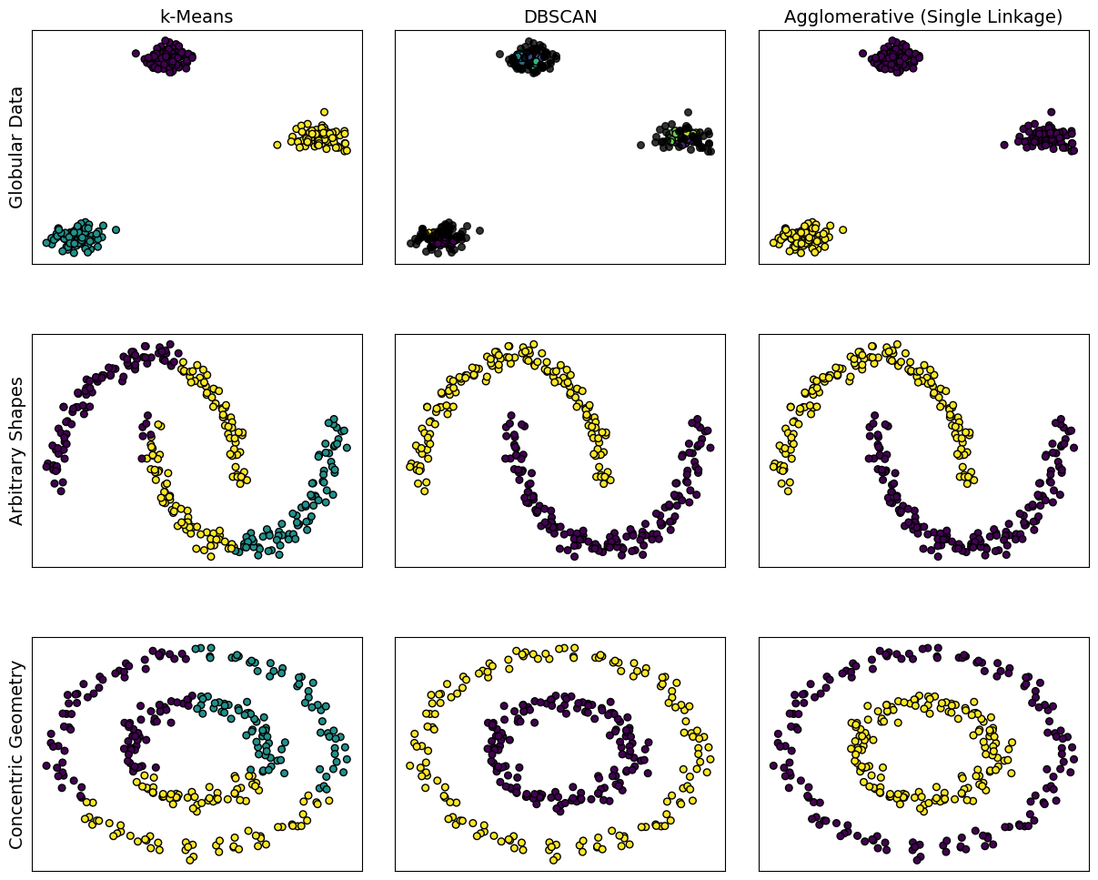
References
Ester, Martin, Hans-Peter Kriegel, Jörg Sander, Xiaowei Xu, et al. 1996. “A Density-Based Algorithm for Discovering Clusters in Large Spatial Databases with Noise.” In Kdd, 96:226–31. 34.
McQueen, James B. 1967. “Some Methods of Classification and Analysis of Multivariate Observations.” In Symposium on Math. Stat. And Prob., 281–97.