import numpy as np
import matplotlib.pyplot as plt
from diffusers import DDPMScheduler, ScoreSdeVeScheduler1.1.3. Stochastic Differential Equations (SDEs) Formulation
After both Score Matching with Langevin Dynamics (SMLD) and Denoising Diffusion Probabilistic Models (DDPMs) were introduced, research focused on unifying these formulations under the same theoretical basis. For that, it was noted that both approaches used noise to perturb data. With that, a connection with Stochastic Differential Equations (SDEs) was done, extending the corruption process to a continuous version (Song et al. 2021).
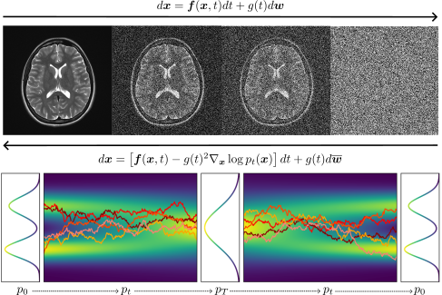
Let \(\{\boldsymbol{x}(t)\}_{t=0}^T\) be a sequence of data \(\boldsymbol x(t) \in \mathbb R^n\) with \(t\in[0,1]\) being a continuous time index. The goal is to obtain a way to sample \(\boldsymbol{x}(0) \sim p_0\), for which \(p_0\) is the data distribution, while \(p_T\) is the prior distribution. The diffusion process can be described as the solution of an Itô SDE: \[ d\boldsymbol{x} = \boldsymbol{f}(\boldsymbol{x}, t) dt + g(t)d\boldsymbol{w}, \tag{1}\] where \(\boldsymbol{w} \in \mathbb R^n\) is the Wiener process, \(\boldsymbol{f}: \mathbb R^{n \times 1} \to \mathbb R^n\) is the drift coefficient of \(\boldsymbol{x}(t)\) and \(g : \mathbb R \to \mathbb R\) is the diffusion coefficient of \(\boldsymbol{x}(t)\). To denote the probability density of \(\boldsymbol{x}(t)\) the notation \(p_t\) is going to be used, which also holds for the transition kernels \(p_{st} (\boldsymbol{x}(s) \mid \boldsymbol{x}(t))\), with \(0\leq s < t \leq T\).
Then, by taking \(\boldsymbol{x}(T) \sim p_T\) and reversing the diffusion process, samples can be obtained from the data distribution. This is modelled by a reverse diffusion process, given by: \[ d\boldsymbol{x} = \left[\boldsymbol{f}(\boldsymbol{x}, t) - g(t)^2 \nabla_{\boldsymbol{x}} \log p_t(\boldsymbol{x})\right] dt + g(t)d\boldsymbol{\overline w}, \tag{2}\] where \(\boldsymbol{\overline w} \in \mathbb R^n\) is the Wiener process running from \(T\) to \(0\). To reverse the process, however, one needs to approximate the score function \(\nabla_{\boldsymbol{x}} \log p_t(\boldsymbol{x}): \mathbb R^{n \times 1} \to \mathbb R^n\) at each time step \(t\). The general diffusion framework is schematically depicted in Figure 1.
Observing the transition kernel from SMLD, which is defined as: \[ \boldsymbol{x}_t = \boldsymbol{x}_{t-1} + \sqrt{\sigma_t^2 - \sigma_{t-1}^2} \boldsymbol{z}_{t-1}. \tag{3}\] In the limit of \(T\to \infty\), the expression becomes a continuous stochastic process, given by: \[ d\boldsymbol{x} = \sqrt{\frac{d[\sigma(t)^2]}{dt}} d\boldsymbol{w}. \tag{4}\] Analogously for the DDPM transition kernel: \[ \boldsymbol{x}_t = \sqrt{1 - \beta_t} \boldsymbol{x}_{t-1} + \sqrt{\beta_t} \boldsymbol{z}_{t-1}, \tag{5}\] with \(T\to \infty\): \[ d\boldsymbol{x} = -\frac{1}{2}\beta(t) \boldsymbol{x} dt + \sqrt{\beta(t)}d\boldsymbol{w}. \tag{6}\] Therefore, it was possible to observe that both SMLDs and DDPMs were particular discretization cases for a more general diffusion process framework. The SMLD increases the variance as time goes to infinity, so it is called a Variance Exploding (VE) SDE, while the DDPM is a Variance Preserving (VP) SDE. In the work, the authors introduced a sub-VP SDE, given by: \[ d\boldsymbol{x} = -\frac{1}{2}\beta(t) \boldsymbol{x} dt + \sqrt{\beta(t)\left(1 - \exp\left(-2\int^t_0\beta(s)ds\right)\right)}d\boldsymbol{w}. \tag{7}\] This was called a sub-VP SDE because at each time step \(t\), its variance is bounded by the VP equation.
The objective functions of both SMLDs and DDPMs were also unified. That is, the general form of the continuous objective function can be written as: \[ \mathcal{L}(\boldsymbol{\theta}) = \mathbb{E}_{t, \boldsymbol{x}_0, \boldsymbol{\epsilon}} \left[ \lambda(t) \left\| \boldsymbol{s}_{\boldsymbol{\theta}}(\boldsymbol{x}_t, t) + \frac{\boldsymbol{\epsilon}}{\sigma_t} \right\|_2^2 \right], \tag{8}\] where \(\lambda(t) : \mathbb R \to \mathbb R\) is a weighting function introduced to balance the gradient magnitudes across different noise scales. If one sets \(\lambda(t) = \sigma_t^2\) to the respective forward processes of SMLDs and DDPMs, one gets their original objective functions.
It was also shown that every diffusion process has a deterministic process that shares the same marginal probability densities \(p_t(\boldsymbol{x})\) for all \(t\). This is modelled by an Ordinary Differential Equation (ODE), known as the Probability Flow ODE, given by: \[ d\boldsymbol{x} = \left[\boldsymbol{f}(\boldsymbol{x}, t) - \frac{1}{2}g(t)^2 \nabla_{\boldsymbol{x}} \log p_t(\boldsymbol{x})\right] dt. \tag{9}\] Because this formulation removes the stochastic Wiener process, the generative trajectory becomes entirely deterministic.
The SDE formulation also decoupled the learning process of the prior with the inference time sampling process. While DDPM used Ancestral Sampling and SMLD employed Annealed Langevin Dynamics, the authors
The SDE formulation also decoupled the training of the generative model from the inference-time sampling process. While frameworks relied on fixed schemes – such as DDPM using Ancestral Sampling and SMLD employing Annealed Langevin Dynamics – the continuous-time formulation demonstrated that given a trained score network, different samplers could be used to generate the data, without retraining the model. In the work, a new Predictor-Corrector (PC) algorithm was also proposed.
Code
Importing the packages.
Instantiating the schedulers.
T = 1000
t_continuous = np.linspace(0, 1, T)

vp_scheduler = DDPMScheduler(
    num_train_timesteps=T,
    beta_start=0.0001,
    beta_end=0.02,
    beta_schedule="linear"
)

ve_scheduler = ScoreSdeVeScheduler(
    num_train_timesteps=T,
    sigma_min=0.01,
    sigma_max=50.0
)

alphas_cumprod = vp_scheduler.alphas_cumprod.numpy()
var_vp = 1.0 - alphas_cumprod

var_sub_vp = (1.0 - alphas_cumprod) ** 2

if hasattr(ve_scheduler, 'discrete_sigmas'):
    sigmas = ve_scheduler.discrete_sigmas.numpy()
else:
    sigmas = ve_scheduler.sigmas.numpy()

var_ve = sigmas ** 2
Plotting the variances from different SDEs.
fig, axes = plt.subplots(1, 2, figsize=(15, 5))

axes[0].plot(t_continuous, var_ve, color='crimson', linewidth=2.5)
axes[0].set_title("VE SDE", fontsize=14)
axes[0].set_xlabel(r"$t$", fontsize=12)
axes[0].set_ylabel("Marginal Variance", fontsize=12)
axes[0].grid(True, alpha=0.3)

axes[1].plot(t_continuous, var_vp, label='VP SDE', color='blue', linewidth=2.5)
axes[1].plot(t_continuous, var_sub_vp, label='sub-VP SDE', color='purple', linestyle='--', linewidth=2.5)
axes[1].set_title("VP SDEs", fontsize=14)
axes[1].set_xlabel(r"$t$", fontsize=12)
axes[1].set_ylabel("Marginal Variance", fontsize=12)
axes[1].grid(True, alpha=0.3)
axes[1].legend(fontsize=12)

plt.tight_layout()
plt.show()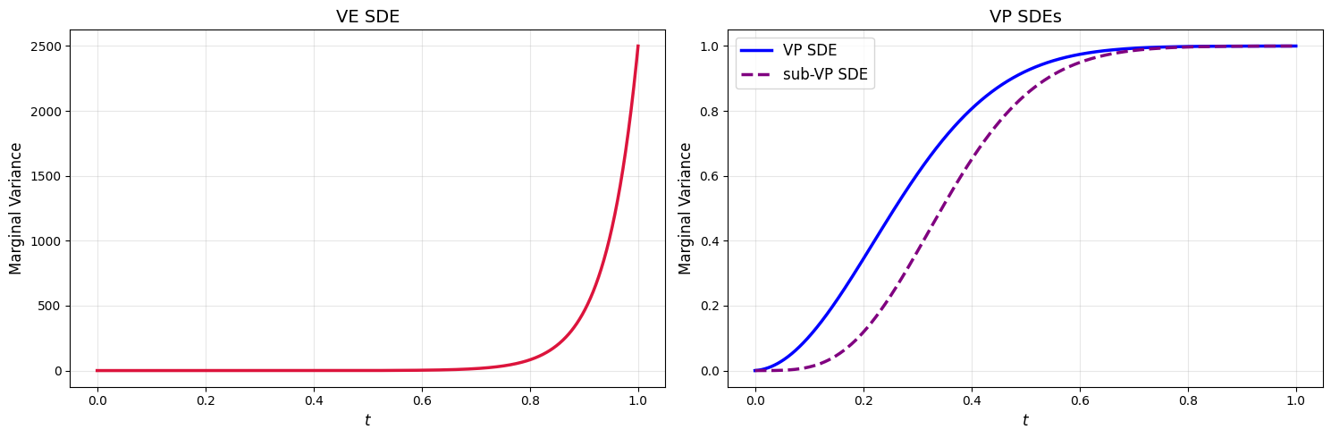
References
Song, Yang, Jascha Sohl-Dickstein, Diederik P Kingma, Abhishek Kumar, Stefano Ermon, and Ben Poole. 2021. “Score-Based Generative Modeling Through Stochastic Differential Equations.” In International Conference on Learning Representations.