import numpy as np
import matplotlib.pyplot as plt
from sklearn.preprocessing import MaxAbsScaler, MinMaxScaler, StandardScaler1.1. Pre-Processing
Before feeding the data to a model, it is usually necessary to pre-process it. This is necessary due to the mathematical formulation of these models, where some of them might require data to follow specific patterns. Here, the following pre-processing strategies are going to be presented: normalization, encoding and feature selection.
Normalization
Normalization is a class of transformations that make features present more uniform statistics. The first approach for normalizing data is the absolute maximum normalization. This technique takes the a set of features \(\boldsymbol X \in \mathbb R^{N\times n}\), where \(N\) is the number of observations and \(n\) is the number of features, and applies the following transformation: \[ \boldsymbol{\tilde X} = \frac{\boldsymbol{X}}{\max\mid\boldsymbol{X}\mid}, \tag{1}\] where \(\boldsymbol{\tilde X}\) is the normalized set of features. This normalization scales the data between \(-1\) and \(1\), while preserving sparsity. Note that the maximum is taken feature-wise, and so is the division.
Another type of normalization is the \(\min-\max\) normalization, which scales the data between \(0\) and \(1\), where the minimum value of the original data is mapped to \(0\), and the maximum to \(1\). It is given by: \[ \boldsymbol{\tilde X} = \frac{\boldsymbol{X} - \min(\boldsymbol{X})}{\max(\boldsymbol{X}) - \min(\boldsymbol{X})}. \tag{2}\] Note that unlike absolute maximum normalization, \(\min-\max\) normalization does not preserve sparsity.
Finally, standard normalization scales the data to so that each feature has a standard deviation of \(1\) and a mean of \(0\). The transformation is given by: \[ \boldsymbol{\tilde X} = \frac{\boldsymbol{X} - \boldsymbol{\mu}_{\boldsymbol{X}}}{\boldsymbol{\sigma}_{\boldsymbol{X}}}, \tag{3}\] where \(\boldsymbol{\mu}_{\boldsymbol{X}}\) are the mean values of the features and \(\boldsymbol{\sigma}_{\boldsymbol{X}}\) are the standard deviations.
Code: Normalization
Here, synthetic data is going to be normalized, in order to compare the different transformations explained. Importing packages.
Generating and printing data minimum and maximum.
feature_1 = np.random.normal(500000, 50000, 100)
feature_2 = np.random.normal(3, 1, 100)

X = np.column_stack((feature_1, feature_2))

print(f"Minimum: {X.min(axis=0)}")
print(f"Maximum: {X.max(axis=0)}")
Minimum: [3.44361495e+05 7.88805078e-02]
Maximum: [6.15555239e+05 5.18227783e+00]Applying absolute maximum absolute normalization.
max_abs_scaler = MaxAbsScaler()
X_maxabs = max_abs_scaler.fit_transform(X)

print(f"Minimum: {X_maxabs.min(axis=0)}")
print(f"Maximum: {X_maxabs.max(axis=0)}")
Minimum: [0.55943232 0.0152212 ]
Maximum: [1. 1.]Applying min-max normalization.
min_max_scaler = MinMaxScaler()
X_minmax = min_max_scaler.fit_transform(X)

print(f"Minimum: {X_minmax.min(axis=0)}")
print(f"Maximum: {X_minmax.max(axis=0)}")
Minimum: [0. 0.]
Maximum: [1. 1.]Applying standard normalization.
std_scaler = StandardScaler()
X_std = std_scaler.fit_transform(X)

print(f"Mean: {X_std.mean(axis=0)}")
print(f"Std:  {X_std.std(axis=0)}")
Mean: [ 3.74367204e-15 -5.90638649e-16]
Std: [1. 1.]Plotting the data with different normalizations.
fig, axes = plt.subplots(2, 2, figsize=(10, 10))
axes = axes.ravel()

axes[0].scatter(X[:, 0], X[:, 1], alpha=0.7, color='red')
axes[0].set_title("Original Data")
axes[0].set_xlabel("Feature 1")
axes[0].set_ylabel("Feature 2")

axes[1].scatter(X_maxabs[:, 0], X_maxabs[:, 1], alpha=0.7, color='green')
axes[1].set_title("Maximum Absolute Normalization")
axes[1].set_xlabel("Feature 1")
axes[1].set_ylabel("Feature 2")

axes[2].scatter(X_minmax[:, 0], X_minmax[:, 1], alpha=0.7, color='green')
axes[2].set_title("Min-Max Normalization")
axes[2].set_xlabel("Feature 1")
axes[2].set_ylabel("Feature 2")

axes[3].scatter(X_std[:, 0], X_std[:, 1], alpha=0.7, color='blue')
axes[3].set_title("Standard Normalization")
axes[3].set_xlabel("Feature 1")
axes[3].set_ylabel("Feature 2")

plt.tight_layout()
plt.show()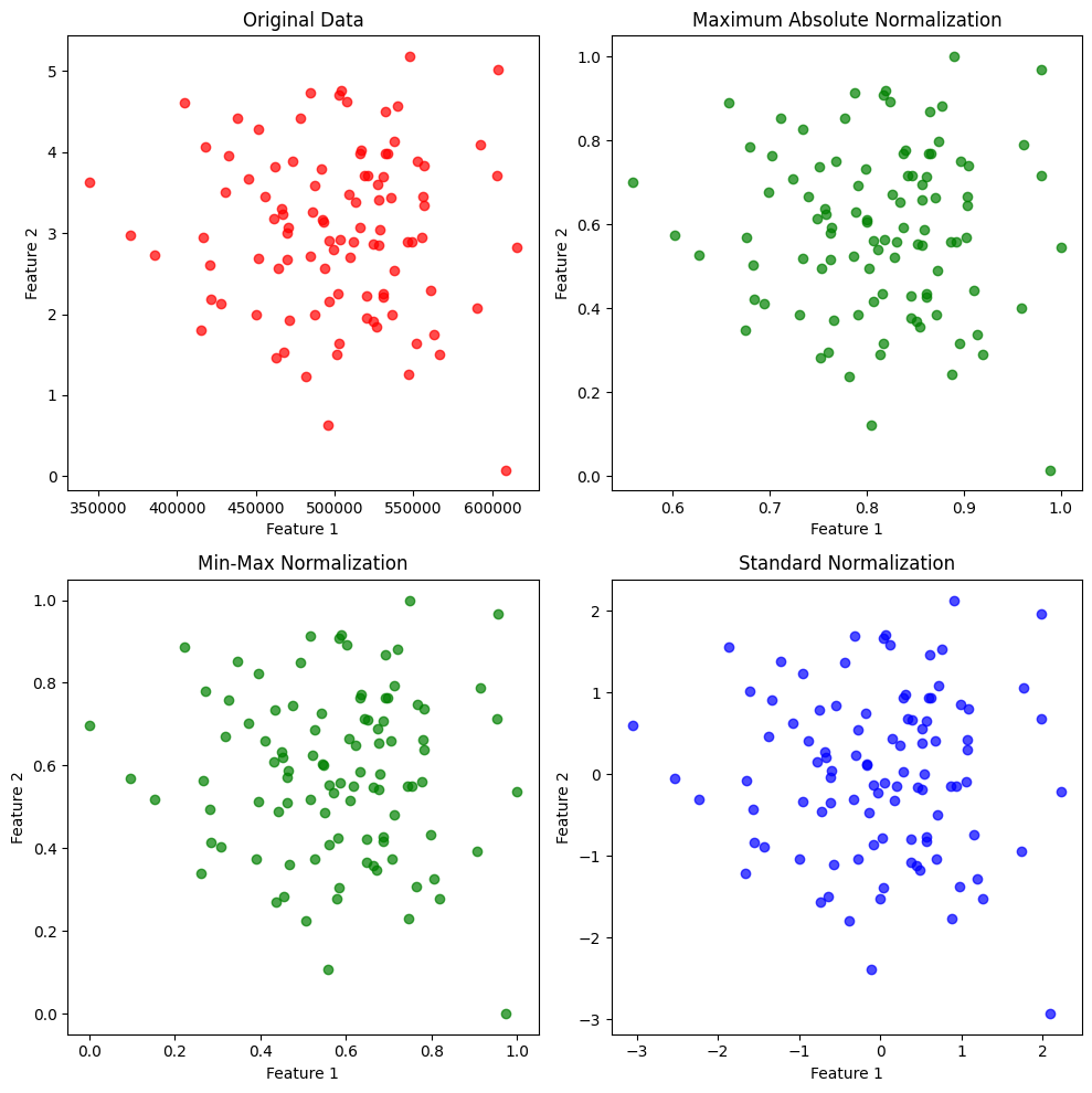
Encoding
Another important part of pre-processing is encoding features that are not numerical. This envolves finding good representations for features that might be stored as strings, for example. When there is some sense of order in the feature, the ordinal encoder is used. It converts the \(m\) original classes into integers, keeping the order. On the other hand, if there is no order, the data is passed through a one-hot encoder, which converts the original \(m\) classes into \(m\) new features, where the columns are sparse, only containing \(1\) when the observations belongs to the specific class.
Code: Encoding
Feature Selection
In some cases, the dataset has numerous features, resulting in complex and computationally expensive models. Therefore, it is interesting to select a small subset of features to decrease the computational cost of the trained model. This selection is important to avoid the curse of dimensionality, in which the increase of features in the model worsens its performance.
The first strategy is to eliminate features by variance. When a feature does not vary throughout observations, it does not add new information to the model, therefore, it can be excluded. Similarly, one can define a variance threshold for eliminating features.
A more advanced approach is to use the Variance Inflation Factor (VIF) algorithm. It removes features based on their multicollinearity with other features. That is, if one feature is a linear combination of other ones, it is removed. For each feature \(x_j \in \boldsymbol{X}\), the VIF trains a linear regression with \(x_j\) as a target. The coefficient of determination \(R^2\) of the final model is used to calculate the VIF coefficient: \[ \text{VIF}(x_j) = \frac{1}{1-R_j^2}. \tag{4}\] If this coefficient is equal to \(1\), there is no multicollinearity, while higher values indicate correlation. With that, given a threshold – generally \(5\) or \(10\) –, features can be removed.