1.1.2. Denoising Diffusion Probabilistic Models (DDPM)

Following the Score Matching with Langevin Dynamics (SMLD), Denoising Diffusion Probabilistic Models (DDPMs) (Ho, Jain, and Abbeel 2020) formulated a Diffusion Models (DMs) as two separate processes. The forward, or diffusion process was defined as a fixed Markov chain that increasingly added noise to the original data \(\boldsymbol{x}_0\in \mathbb R^n\), being described as: \[ q(\boldsymbol{x}_{1:T}\mid \boldsymbol{x}_0) = \prod_{t=1}^T q(\boldsymbol{x}_t\mid \boldsymbol{x}_{t-1}), \tag{1}\] where \(T\in \mathbb N\) is the number of states in the chain. Each transition in this process can be expressed as: \[ q(\boldsymbol{x}_t\mid \boldsymbol{x}_{t-1}) = \mathcal N\left(\boldsymbol{x}_t\mid \sqrt{1-\beta_t}\boldsymbol{x}_{t-1}, \beta_t\boldsymbol{I}\right), \tag{2}\] where \(\{\beta_i\}_{i=1}^T\) is a variance schedule, with \(\beta_i \in \mathbb R\). The diffusion process admits sampling any step in the chain directly from the original sample, with the following: \[ \boldsymbol x_t = \sqrt{\overline{\alpha}_t}\boldsymbol x_0 + \sqrt{1 - \overline{\alpha}_t} \boldsymbol \epsilon, \tag{3}\] where \(\alpha_t = 1 - \beta_t\), \(\overline{\alpha}_t = \prod_{s=1}^t \alpha_s\) and \(\boldsymbol{\epsilon}\sim \mathcal N(\boldsymbol{\epsilon}\mid\boldsymbol{0}, \boldsymbol{I})\), with \(\boldsymbol{\epsilon} \in \mathbb R^n\).

The reverse process was defined as a Markov chain where the Gaussian transitions were learned via a parametrized Neural Network (NN). Starting with \(\boldsymbol x_T\in \mathbb R^n\), where \(\boldsymbol{x}_T \sim \mathcal{N}(\boldsymbol{x}_T \mid \boldsymbol{0}, \boldsymbol{I})\), the NN parametrized by \(\boldsymbol{\theta}\) approximated the following chain: \[ p_{\boldsymbol{\theta}}\left(\boldsymbol{x}_{0:T}\right) = p(\boldsymbol x_T) \prod_{t=1}^T p_{\boldsymbol \theta}(\boldsymbol x_{t-1}\mid \boldsymbol x_t). \tag{4}\] Each transition step is expressed as: \[ p_{\boldsymbol{\theta}}(\boldsymbol{x}_{t-1} \mid \boldsymbol{x}_{t}) = \mathcal N\left(\boldsymbol{x}_{t-1}\mid {\boldsymbol\mu}_{\boldsymbol{\theta}}(\boldsymbol{x}_t, t), {\boldsymbol\Sigma}_{\boldsymbol{\theta}}(\boldsymbol{x}_t, t)\right). \tag{5}\] That is, the DM learned the mean \({\boldsymbol\mu}_{\boldsymbol{\theta}}(\boldsymbol{x}_t, t) : \mathbb R^{n \times 1} \to \mathbb R^n\) and variance \({\boldsymbol\Sigma}_{\boldsymbol{\theta}}(\boldsymbol{x}_t, t) : \mathbb R^{n \times 1} \to \mathbb R^n\) to reverse the noise from \(\boldsymbol{x}_{t}\) to \(\boldsymbol{x}_{t-1}\). To achieve this, the model was conditioned on the time step \(t\).

The NN was trained to minimize the negative log-likelihood of the data. Making some algebraic steps: \[ \begin{aligned} \mathcal L(\boldsymbol{\theta}) &= \mathbb E\left[ -\log p_{\boldsymbol{\theta}} (\boldsymbol{x}_0)\right] \leq \mathbb E_q\left[- \log\frac{p_{\boldsymbol{\theta}} (\boldsymbol x_{0:T})}{q(\boldsymbol{x}_{1:T} \mid \boldsymbol{x}_0)}\right] \\ &= \mathbb E_q\left[- \log p(\boldsymbol{x}_T) - \sum_{t\geq 1} \log\frac{p_{\boldsymbol{\theta}} (\boldsymbol x_{t-1} \mid \boldsymbol{x}_t)}{q(\boldsymbol{x}_{t} \mid \boldsymbol{x}_{t-1})}\right] \\ &= \mathbb E_q\left[- \log p(\boldsymbol{x}_T) - \log \frac{p_{\boldsymbol{\theta}} (\boldsymbol x_{0} \mid \boldsymbol{x}_1)}{q(\boldsymbol{x}_{1} \mid \boldsymbol{x}_{0})} - \sum_{t> 1}\log \frac{p_{\boldsymbol{\theta}} (\boldsymbol x_{t-1} \mid \boldsymbol{x}_t)}{q(\boldsymbol{x}_{t} \mid \boldsymbol{x}_{t-1})}\right]. \end{aligned} \tag{6}\] Applying Bayes’ Theorem to the forward Markov chain: \[ \begin{aligned} &= \mathbb E_q\left[- \log p(\boldsymbol{x}_T) - \log \frac{p_{\boldsymbol{\theta}} (\boldsymbol x_{0} \mid \boldsymbol{x}_1)}{q(\boldsymbol{x}_{1} \mid \boldsymbol{x}_{0})} - \sum_{t> 1} \log \frac{p_{\boldsymbol{\theta}} (\boldsymbol x_{t-1} \mid \boldsymbol{x}_t)q(\boldsymbol x_{t-1} \mid \boldsymbol{x}_0)}{q(\boldsymbol{x}_{t-1} \mid \boldsymbol{x}_{t}, \boldsymbol{x}_0) q(\boldsymbol{x}_{t} \mid \boldsymbol{x}_{0})} \right] \\ &= \mathbb E_q\left[- \log \frac{p(\boldsymbol{x}_T)}{q(\boldsymbol{x}_T \mid \boldsymbol{x}_0)} - \log p_{\boldsymbol{\theta}} (\boldsymbol x_{0} \mid \boldsymbol{x}_1)- \sum_{t> 1} \log \frac{p_{\boldsymbol{\theta}} (\boldsymbol x_{t-1} \mid \boldsymbol{x}_t)}{q(\boldsymbol{x}_{t-1} \mid \boldsymbol{x}_{t}, \boldsymbol{x}_0)}\right] \\ &= \mathbb E_q\bigg[ \underbrace{D_{\text{KL}} \bigg(q(\boldsymbol{x}_T \mid \boldsymbol{x}_0) \parallel p(\boldsymbol{x}_T) \bigg)}_{\mathcal L_T} \underbrace{- \log p_{\boldsymbol{\theta}} (\boldsymbol x_{0} \mid \boldsymbol{x}_1)}_{\mathcal L_0} \\ &\qquad \qquad \qquad + \sum_{t> 1} \underbrace{D_{\text{KL}} \bigg(q(\boldsymbol{x}_{t-1} \mid \boldsymbol{x}_{t}, \boldsymbol{x}_0) \parallel p_{\boldsymbol{\theta}}(\boldsymbol{x}_{t-1} \mid \boldsymbol{x} _t) \bigg)}_{\mathcal L_{t-1}}\bigg], \end{aligned} \tag{7}\] where \(D_{\text{KL}}\) is the Kullback-Leibler divergence. Note that by fixing the forward process, the term \(\mathcal L_T\) does not depend on \(\boldsymbol{\theta}\) and can therefore be ignored. For the \(\mathcal L_{1:T-1}\) terms, the variance of the NN is fixed to \({\boldsymbol\Sigma}_{\boldsymbol{\theta}}(\boldsymbol{x}_t, t) = \sigma_t^2\boldsymbol{I} = \beta_t \boldsymbol{I}\).

With the fixed variance, the KL divergence in the \(\mathcal{L}_{t-1}\) terms compares two Gaussian distributions. This simplifies to the mean squared error between their means. The posterior \(q(\boldsymbol{x}_{t-1} \mid \boldsymbol{x}_t, \boldsymbol{x}_0)\) is also a Gaussian, therefore, minimizing \(\mathcal{L}_{t-1}\) is equivalent to minimizing the difference between the true posterior mean \(\tilde{\boldsymbol{\mu}}_t \in \mathbb R^n\) and the NN’s predicted mean \(\boldsymbol{\mu}_{\boldsymbol{\theta}} \in \mathbb R^n\): \[ \mathcal L_{t-1} = \mathbb E_q \left[ \frac{1}{2\sigma_t^2} \left\| \tilde{\boldsymbol{\mu}}_t(\boldsymbol{x}_t, \boldsymbol{x}_0) - \boldsymbol{\mu}_{\boldsymbol{\theta}}(\boldsymbol{x}_t, t) \right\|^2 \right] + C, \tag{8}\] where \(C \in \mathbb R\) is a constant independent of \(\boldsymbol{\theta}\). With some reparametrization tricks, it was possible to show that these terms can be expressed as: \[ \mathcal L_{t-1} = \mathbb E_{\boldsymbol{x}_0, \boldsymbol{\epsilon}} \left[ \frac{\beta_t^2}{2\sigma_t^2 \alpha_t (1 - \overline{\alpha}_t)} \left\| \boldsymbol{\epsilon} - \boldsymbol{\epsilon}_{\boldsymbol{\theta}}(\boldsymbol{x}_t, t) \right\|^2 \right], \tag{9}\] where \(\boldsymbol{\epsilon}_{\boldsymbol{\theta}}(\boldsymbol{x}_t, t) : \mathbb R^{n \times 1} \to \mathbb R^n\) is the noise predicted by the NN. It was observed that ignoring the weighting term lead to better results. This results in the final simplified objective function used to train DDPMs: \[ \mathcal L(\boldsymbol{\theta}) = \mathbb E_{t, \boldsymbol{x}_0, \boldsymbol{\epsilon}} \left[ \left\| \boldsymbol{\epsilon} - \boldsymbol{\epsilon}_{\boldsymbol{\theta}}(\boldsymbol{x}_t, t) \right\|^2 \right]. \tag{10}\]

To generate samples from \(p_0\), DDPM employed the Ancestral Sampling algorithm to iteratively denoise random noise \(\boldsymbol x_T \sim p_T\).

Code

Importing the packages.

import torch
import numpy as np
import matplotlib.pyplot as plt
from torchvision import transforms
from torchvision.datasets import MNIST
from diffusers import DDPMScheduler

Plotting the noise schedule of DDPM.

T = 1000
scheduler = DDPMScheduler(num_train_timesteps=T, beta_schedule="linear")

betas = scheduler.betas.numpy()
alphas = scheduler.alphas.numpy()
alphas_cumprod = scheduler.alphas_cumprod.numpy()

steps = np.arange(1, T + 1)

fig, axes = plt.subplots(1, 3, figsize=(15, 4))
axes[0].plot(steps, betas, color="crimson", linewidth=2)
axes[0].set_ylabel(r"$\beta_t$", fontsize=14)
axes[0].set_xlabel(r"$t$")

axes[1].plot(steps, alphas, color="blue", linewidth=2)
axes[1].set_ylabel(r"$\alpha_t$", fontsize=14)
axes[1].set_xlabel(r"$t$")

axes[2].plot(steps, alphas_cumprod, color="purple", linewidth=2)
axes[2].set_ylabel(r"$\bar{\alpha}_t$", fontsize=14)
axes[2].set_xlabel(r"$t$")

plt.tight_layout()
plt.show()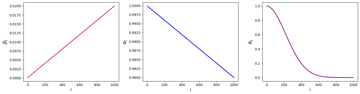

Showing the diffusion process.

dataset = MNIST(root="./data", train=True, download=True, transform=transforms.ToTensor())
x0, _ = dataset[0]
x0 = x0.unsqueeze(0) * 2.0 - 1.0

selected_t = [0, 100, 300, 600, 999]
fig, axes = plt.subplots(1, len(selected_t), figsize=(16, 3))

epsilon = torch.randn_like(x0)

for i, t in enumerate(selected_t):
    if t == 0:
        xt = x0
        title = r"Original $\mathbf{x}_0$"
    else:
        t_tensor = torch.tensor([t], dtype=torch.long)
        xt = scheduler.add_noise(x0, epsilon, t_tensor)
        title = r"$t=$" + f"{t}"

    img = (xt.squeeze().numpy() + 1.0) / 2.0
    axes[i].imshow(img, cmap="gray")
    axes[i].set_title(title, fontsize=12)
    axes[i].axis("off")

plt.show()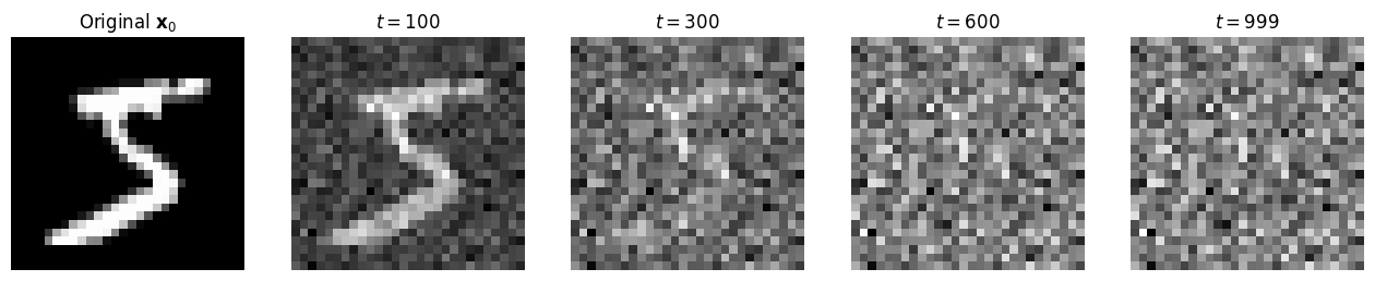

Source: ddpm.ipynb

References

Ho, Jonathan, Ajay Jain, and Pieter Abbeel. 2020. “Denoising Diffusion Probabilistic Models.” Advances in Neural Information Processing Systems 33: 6840–51.