import torch
import matplotlib.pyplot as plt
from diffusers import (
    DDPMPipeline,
    DDPMScheduler,
    ScoreSdeVePipeline,
    ScoreSdeVeScheduler
)2.1. Samplers based on Stochastic Differential Equations (SDEs)
One approach to sampling data from a diffusion generative model is to simulate the reverse diffusion Stochastic Differential Equation (SDE). Let the reverse SDE be: \[ d\boldsymbol{x} = \left[\boldsymbol{f}(\boldsymbol{x}, t) - g(t)^2 \nabla_{\boldsymbol{x}} \log p_t(\boldsymbol{x})\right] dt + g(t)d\boldsymbol{\overline w}, \tag{1}\] where \(\boldsymbol{f}(\cdot, t) : \mathbb R^{n \times 1} \to \mathbb R^n\) is the drift coefficient of \(\boldsymbol{x}(t) \in \mathbb R^n\), \(g(t): \mathbb R \to \mathbb R\) is the diffusion coefficient of \(\boldsymbol{x}(t)\) and \(\boldsymbol{\overline w} \in \mathbb R^n\) is the Wiener process running from \(T\) to \(0\). Then, by discretizing Equation 1, one can iteratively move from \(p_T\) to \(p_0\), effectively sampling from the data distribution given an initial tractable distribution. One important aspect from this approach is that trajectories are stochastic, that is, the same initial noise sample can lead to different generated samples.
Annealed Langevin Dynamics
The Annealed Langevin Dynamics method was proposed in Score-Matching with Langevin Dynamics (SMLD) (Song and Ermon 2019) as a sampling algorithm for SMLD. Let the score network be \(\boldsymbol{s}_{\boldsymbol{\theta}} : \mathbb R^{n \times 1} \to \mathbb R^n\), \(T \in \mathbb N\) be the number of noise levels and \(\boldsymbol{x}_T \in \mathbb R^n\) be noise sampled from \(\boldsymbol{x}_T \sim \mathcal{N}(\boldsymbol{0}, \sigma_T^2 \boldsymbol{I})\), where \(\sigma_T \in \mathbb R\) is the highest noise level. Starting from the initial noise sample, the algorithm iteratively walks along the estimated score vectors, moving towards regions of higher data density. To prevent the generated data from collapsing into local maxima, a stochastic step is performed at each iteration. For a given noise level \(\sigma_t\), the algorithm performs \(M\) gradient steps in the direction of the estimated score. The update rule for the \(m\)-th inner step is given by: \[ \boldsymbol{x}_{t}^{m} = \boldsymbol{x}_{t}^{m-1} + \frac{\sigma'_t}{2} \boldsymbol{s}_{\boldsymbol{\theta}} \left(\boldsymbol{x}_{t}^{m-1}, \sigma_t \right) + \sqrt{\sigma'_t}\boldsymbol{\epsilon}^{m-1}, \tag{2}\] where \(\sigma'_t = \kappa \cdot (\sigma_t^2 / \sigma_1^2)\) is the step size corresponding to the current noise scale \(\sigma_t\) with fixed parameter \(\kappa\), and \(\boldsymbol \epsilon \in \mathbb R^n\) with \(\boldsymbol{\epsilon}^{m-1} \sim \mathcal{N}(\boldsymbol{0}, \boldsymbol{I})\). After \(M\) steps, the noise level is annealed to \(\sigma_{t-1}\), and the process repeats until \(\sigma_1\). Algorithm 1 presents the Annealed Langevin Dynamic Algorithm.
\begin{algorithm} \caption{Annealed Langevin Dynamics} \begin{algorithmic} \REQUIRE Score network $\boldsymbol{s}_{\boldsymbol{\theta}}$, noise levels $\{\sigma_t\}_{t=1}^{T}$, step-size parameter $\kappa$, number of Langevin steps $M$ \STATE $\boldsymbol{x}_T \sim \mathcal{N}(\boldsymbol{0}, \sigma_T^2\boldsymbol{I})$ \FOR{$t = T,\ldots,1$} \STATE $\sigma'_t \gets \kappa \cdot \left(\frac{\sigma_t^2}{\sigma_1^2}\right)$ \STATE $\boldsymbol{x}_t^0 \gets \boldsymbol{x}_t$ \FOR{$m = 1,\ldots,M$} \STATE $\boldsymbol{\epsilon}^{m-1} \sim \mathcal{N}(\boldsymbol{0},\boldsymbol{I})$ \STATE $\boldsymbol{x}_t^m \gets \boldsymbol{x}_t^{m-1} + \frac{\sigma'_t}{2} \boldsymbol{s}_{\boldsymbol{\theta}} \left(\boldsymbol{x}_t^{m-1},\sigma_t\right) + \sqrt{\sigma'_t}\boldsymbol{\epsilon}^{m-1}$ \ENDFOR \IF{$t > 1$} \STATE $\boldsymbol{x}_{t-1} \gets \boldsymbol{x}_t^M$ \ELSE \STATE $\boldsymbol{x}_1 \gets \boldsymbol{x}_t^M$ \ENDIF \ENDFOR \STATE $\boldsymbol{x}_0 \gets \boldsymbol{x}_1$ \RETURN $\boldsymbol{x}_0$ \end{algorithmic} \end{algorithm}
Ancestral Sampling
The Ancestral Sampling method was proposed in Denoising Diffusion Probabilistic Models (DDPMs) (Ho, Jain, and Abbeel 2020) as its sampling algorithm. Let the noise network be \(\boldsymbol{\epsilon}_{\boldsymbol{\theta}} (\boldsymbol x_t, t): \mathbb R^{n \times 1} \to \mathbb R^n\), \(T \in \mathbb N\) be the number of reverse diffusion steps, and \(\boldsymbol{x}_T \in \mathbb R^n\) be noise sampled from \(\boldsymbol{x}_T \sim \mathcal{N}(\boldsymbol{0}, \boldsymbol{I})\). Additionally, let the diffusion SDE from DDPM be defined as: \[ d\boldsymbol{x} = -\frac{1}{2}\beta(t) \boldsymbol{x} dt + \sqrt{\beta(t)}d\boldsymbol{w}, \tag{3}\] where \(\beta(t): \mathbb R \to \mathbb R_{>0}\) is a parameter from the noise schedule. Then, Ancestral Sampling iteratively follows: \[ \boldsymbol{x}_{t-1} = \frac{1}{\sqrt{\alpha_t}}\left(\boldsymbol{x}_t - \frac{\beta_t}{\sqrt{1-\overline{\alpha}_t}} \boldsymbol{\epsilon}_{\boldsymbol{\theta}}(\boldsymbol{x}_t, t)\right) + \sigma_t\boldsymbol{\epsilon}, \tag{4}\] where the noise \(\boldsymbol \epsilon \in \mathbb R^n\) is sampled as \(\boldsymbol{\epsilon} \sim \mathcal{N}(\boldsymbol{0}, \boldsymbol{I})\) for \(t > 1\), \(\alpha_t = 1-\beta_t\), \(\overline{\alpha}_t = \prod_{s=1}^{t}\alpha_s\), and \(\sigma_t^2 = \frac{1-\overline{\alpha}_{t-1}}{1-\overline{\alpha}_t}\beta_t\). At the final step when \(t = 1\), \(\boldsymbol{\epsilon} = \boldsymbol{0}\) was set to output the deterministic mean, as adding noise at the very end would degrade the final image. The algorithm is presented in Algorithm 2.
\begin{algorithm} \caption{Ancestral Sampling} \begin{algorithmic} \REQUIRE Noise network $\boldsymbol{\epsilon}_{\boldsymbol{\theta}}$, number of diffusion steps $T$, noise schedule $\{\beta_t\}_{t=1}^{T}$ \STATE $\alpha_t \gets 1-\beta_t$ for $t=1,\ldots,T$ \STATE $\overline{\alpha}_t \gets \prod_{s=1}^{t}\alpha_s$ for $t=1,\ldots,T$ \STATE $\sigma_t^2 \gets \frac{1-\overline{\alpha}_{t-1}} {1-\overline{\alpha}_t}\beta_t, \ \ \forall t\in \{1,\ldots,T\}$ \STATE $\boldsymbol{x}_T \sim \mathcal{N}(\boldsymbol{0},\boldsymbol{I})$ \FOR{$t=T,\ldots,1$} \STATE $\boldsymbol{\mu}_t \gets \frac{1}{\sqrt{\alpha_t}} \left(\boldsymbol{x}_t - \frac{\beta_t}{\sqrt{1-\overline{\alpha}_t}} \boldsymbol{\epsilon}_{\boldsymbol{\theta}}(\boldsymbol{x}_t,t) \right)$ \IF{$t > 1$} \STATE $\boldsymbol{\epsilon} \sim \mathcal{N}(\boldsymbol{0},\boldsymbol{I})$ \ELSE \STATE $\boldsymbol{\epsilon} \gets \boldsymbol{0}$ \ENDIF \STATE $\boldsymbol{x}_{t-1} \gets \boldsymbol{\mu}_t + \sigma_t\boldsymbol{\epsilon}$ \ENDFOR \RETURN $\boldsymbol{x}_0$ \end{algorithmic} \end{algorithm}
Predictor-Corrector (PC)
The SDEs formulation also generalized previous sampling methods into a unified Predictor-Corrector (PC) family of algorithms. These methods are divided into two distinct steps. The first is the predictor, which provides an estimate of the next denoised data point along the reverse diffusion trajectory. Then, the corrector step is applied via a score-based Markov Chain Monte Carlo (MCMC) approach to project the estimate back onto the data manifold. It was noted by the authors that DDPM relied solely on a predictor step, while SMLD relied entirely on a corrector step. Consequently, generalized PC algorithms were proposed for both the Variance Exploding (VE) and Variance Preserving (VP) SDEs, presented respectively in Algorithm 3 and Algorithm 4. These algorithms used the numerical discretization of the reverse-time SDE as the predictor, and Annealed Langevin Dynamics as the corrector.
\begin{algorithm} \caption{VE Predictor-Corrector} \begin{algorithmic} \REQUIRE Score network $\boldsymbol{s}_{\boldsymbol{\theta}}$, noise levels $\{\sigma_t\}_{t=0}^{T}$, corrector step sizes $\{\kappa_t\}_{t=1}^{T}$, number of corrector steps $M$ \STATE $\boldsymbol{x}_T \sim \mathcal{N}(\boldsymbol{0}, \sigma_T^2\boldsymbol{I})$ \FOR{$t = T,\ldots,1$} \STATE $\boldsymbol{\epsilon} \sim \mathcal{N}(\boldsymbol{0}, \boldsymbol{I})$ \STATE $\boldsymbol{x}_{t-1}' \gets \boldsymbol{x}_t + (\sigma_t^2 - \sigma_{t-1}^2) \boldsymbol{s}_{\boldsymbol{\theta}}(\boldsymbol{x}_t, \sigma_t) + \sqrt{\sigma_t^2 - \sigma_{t-1}^2} \boldsymbol{\epsilon}$ \STATE $\boldsymbol{x}_{t-1}^0 \gets \boldsymbol{x}_{t-1}'$ \FOR{$m = 1,\ldots,M$} \STATE $\boldsymbol{\epsilon} \sim \mathcal{N}(\boldsymbol{0}, \boldsymbol{I})$ \STATE $\boldsymbol{x}_{t-1}^m \gets \boldsymbol{x}_{t-1}^{m-1} + \frac{\kappa_{t-1}}{2} \boldsymbol{s}_{\boldsymbol{\theta}}(\boldsymbol{x}_{t-1}^{m-1}, \sigma_{t-1}) + \sqrt{\kappa_{t-1}} \boldsymbol{\epsilon}$ \ENDFOR \STATE $\boldsymbol{x}_{t-1} \gets \boldsymbol{x}_{t-1}^M$ \ENDFOR \RETURN $\boldsymbol{x}_0$ \end{algorithmic} \end{algorithm}
\begin{algorithm} \caption{VP Predictor-Corrector} \begin{algorithmic} \REQUIRE Score network $\boldsymbol{s}_{\boldsymbol{\theta}}$, noise schedule $\{\beta_t\}_{t=1}^{T}$, corrector step sizes $\{\kappa_t\}_{t=1}^{T}$, number of corrector steps $M$ \STATE $\alpha_t \gets 1-\beta_t$ for $t=1,\ldots,T$ \STATE $\boldsymbol{x}_T \sim \mathcal{N}(\boldsymbol{0}, \boldsymbol{I})$ \FOR{$t = T,\ldots,1$} \IF{$t > 1$} \STATE $\boldsymbol{\epsilon} \sim \mathcal{N}(\boldsymbol{0}, \boldsymbol{I})$ \ELSE \STATE $\boldsymbol{\epsilon} \gets \boldsymbol{0}$ \ENDIF \STATE $\boldsymbol{x}_{t-1}' \gets \frac{1}{\sqrt{\alpha_t}} \left( \boldsymbol{x}_t + \beta_t \boldsymbol{s}_{\boldsymbol{\theta}}(\boldsymbol{x}_t, t) \right) + \sqrt{\beta_t} \boldsymbol{\epsilon}$ \STATE $\boldsymbol{x}_{t-1}^0 \gets \boldsymbol{x}_{t-1}'$ \FOR{$m = 1,\ldots,M$} \STATE $\boldsymbol{\epsilon} \sim \mathcal{N}(\boldsymbol{0}, \boldsymbol{I})$ \STATE $\boldsymbol{x}_{t-1}^m \gets \boldsymbol{x}_{t-1}^{m-1} + \frac{\kappa_{t-1}}{2} \boldsymbol{s}_{\boldsymbol{\theta}}(\boldsymbol{x}_{t-1}^{m-1}, t-1) + \sqrt{\kappa_{t-1}} \boldsymbol{\epsilon}$ \ENDFOR \STATE $\boldsymbol{x}_{t-1} \gets \boldsymbol{x}_{t-1}^M$ \ENDFOR \RETURN $\boldsymbol{x}_0$ \end{algorithmic} \end{algorithm}
Code
Importing the packages.
Loading pre-trained models and using Ancestral Sampling and VE PC.
device = "cuda" if torch.cuda.is_available() else "cpu"
vp_pipeline = DDPMPipeline.from_pretrained("google/ddpm-cifar10-32").to(device)

vp_pipeline.scheduler = DDPMScheduler.from_config(vp_pipeline.scheduler.config)
ancestral_image = vp_pipeline(num_inference_steps=1000).images[0]

ve_pipeline = ScoreSdeVePipeline.from_pretrained("google/ncsnpp-celebahq-256").to(device)

ve_pipeline.scheduler = ScoreSdeVeScheduler.from_config(ve_pipeline.scheduler.config)
pc_ve_image = ve_pipeline(num_inference_steps=1000).images[0]
Plotting the results.
fig, axs = plt.subplots(1, 2, figsize=(10, 5))

axs[0].imshow(ancestral_image)
axs[0].set_title("Ancestral Sampling")
axs[1].imshow(pc_ve_image)
axs[1].set_title("VE-PC")

for ax in axs:
    ax.axis("off")
plt.show()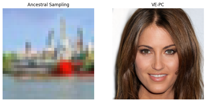
References
Ho, Jonathan, Ajay Jain, and Pieter Abbeel. 2020. “Denoising Diffusion Probabilistic Models.” Advances in Neural Information Processing Systems 33: 6840–51.
Song, Yang, and Stefano Ermon. 2019. “Generative Modeling by Estimating Gradients of the Data Distribution.” Advances in Neural Information Processing Systems 32.